4.4. Radiative Transfer

The photoionization calculations described above are relatively straight forward, provided the internally produced radiation can freely escape the cloud. This is the case in most galactic nebulae, and possibly also in AGN NLR clouds, but not in the BLR, where the optical depth to line and continuum radiation is significant. In this case the calculations must be modified, and the following pages describe some commonly used ways to do so.

4.4.1 Continuum transfer. The internally produced recombination (bound-free) radiation can have a large effect on the degree of ionization by interacting with the gas far from its point of creation. Sophisticated, iterative methods have been developed to account for the propagation of this radiation in the cloud. They depend on the gas distribution and geometry and cannot be applied, in a simple way, to all configurations.

Approximate methods have been developed too, to shorten the calculations and reduce the number of iterations. The "on-the-spot" approximation is based on the assumption that the diffuse radiation is absorbed very close to its point of creation. This is normally a good assumption for the ground level recombination of helium and hydrogen, in nebulae that are very optically thick to the Lyman ionizing radiation. In this case the mean free path of the ground level recombination radiation is very short, and the assumption of local absorption works very well. The approximation is easy to apply since all that is required is to omit recombination to the ground level from the total recombination coefficient in the ionization (3) and thermal equilibrium (10) equations. The method cannot be used for treating recombination to excited levels, where the mean free path of the bound-free radiation is of the order of the cloud size or larger. It also fails near the boundaries of the cloud, where the optical depth to the surface is short even for the ground level recombination radiation.

There are ways to improve this simplified treatment. In the "modified on-the-spot" approximation, a correction factor is applied to each of the recombination coefficients, depending on the optical depth to the surface at the relevant frequency. The application is particularly simple in a slab geometry, where the radiation can be divided into inward going and outward going beams, and only optical depths to two surfaces need to be computed. For example, the recombination coefficient for hydrogen in equation (3), at a point inside the cloud where the Lyman continuum optical depth to the inner (illuminated) side is _in and to the outer side is _out, can be written in the following way:

(25)

where ₁ is the recombination coefficient to n = 1 and _B is the sum of all recombination coefficients to levels with n > 1. The factor a₁, which is of the order of 2, takes into account the oblique escape of the ground level recombination photons and the frequency dependence of the optical depth. A modification of ₂, ₃ etc. can be included in a similar way. Here the frequency dependence of the optical depth must be calculated with great care, which means that a₁ is a strong function of the location in the cloud.

In a second approximation, named "outward only", the locally produced diffuse radiation is added to the incident flux and carried into the cloud in one, or more directions. Its obvious limitations is near the illuminated surface, where no diffuse radiation is allowed to escape. The process puts much of the heat deep in the cloud, causing an unrealistic temperature structure.

The free-free optical depth is never very large and the above approximate transfer methods are not adequate in this case. In many cases the optical depth is so small that no correction term is required. In other cases the free-free optical depth, (ff) must be calculated at all frequencies and included in the free-free heating integral (11). The free-free cooling rate is then modified using the exp(-h_cut / kT_e) factor mentioned in 4.2.2. This local treatment is only a first order approximation to the rather complex full treatment of the free-free radiation transfer.

4.4.2 Line transfer. Standard radiative transfer techniques require a numerical solution of the radiation field everywhere in the gas. Each individual line profile is divided into several frequency bins, and the redistribution in frequency, following an absorption-emission process, is taken into account at all points. This is successfully applied in stellar atmosphere calculations, where conditions are close to LTE. Under such conditions, the local temperature and the level populations are not very sensitive to the emitted line flux and good solutions are obtained even when a small number of transitions are considered.

This is not the case in gaseous nebulae, where conditions are far from LTE, and a complete solution of the statistical equilibrium equations is required in order to calculate the temperature. Realistic photoionization calculations for AGN clouds involved the computation of several hundred emission lines, the large majority of which are optically thick. Neglecting some lines in the energy balance calculations, for the sake of treating the transfer of others in a more complete way, may result in a poor estimate of the kinetic temperature and wrong line ratios. Combining the two types of treatments, by solving the full radiative transfer in all lines, is beyond the capability of the most sophisticated computer codes available. We are thus faced with the choice of treating the radiative transfer in detail, at the expense of the atomic physics, or vice versa.

The alternative, so far preferred in most advanced calculations, is to treat the atomic physics in the most accurate way and use a simplified method for the line transfer. The method is known as the escape probability method and is demonstrated here for the simple case of a two level atom.

Consider a two level atom with an energy separation between the levels of E₁₂ and a normalized line profile , which is assumed to be identical for both absorption and emission. Let I be the radiation intensity and J the intensity averaged over angles and frequencies

(28)

Consider only radiative processes; spontaneous emission, with a rate of n₂A₂₁, absorption, with a rate of n₁B₁₂J and induced emission, with a rate of n₂B₂₁J. The rate equation for the level population is:

(29)

For isotropic line emission the emission coefficient is:

(30)

and the absorption coefficient is:

(31)

where stimulated emission is counted as negative absorption. The line source function, S, is therefore

(32)

where we have made use of the fact that A₂₁ = (2h ³ / c²)B₂₁ and g₁B₁₂ = g₂B₂₁.

Let ₂₁ be the probability of a line photon to escape the cloud and (1 - ₂₁) the probability to be trapped. In the escape probability method we assume that

(33)

which, by using the definition of S (32) and substituting into the rate equation (29), simplifies to

(34)

In the same way the emergent line flux, per unit volume, is:

(35)

This is the essence of the escape probability method. It shows that the equations are similar to the optically thin case except that an effective Einstein coefficient, ₂₁ A₂₁, replaces A₂₁. The method ensures local energy conservation and the local temperature is well determined. The scheme is easily generalized to a many level atom, by replacing A_ji for each transition, by _ji A_ji.

The escape probability approximation gives a correct solution where all scatterings are local and there is little diffusion in space (i.e. the photon is scattered many times close to its point of creation and then escapes the cloud without any further interaction). It is also formally correct for the uniform case, where the temperature and degree of ionization are the same throughout the clouds. In such cases is a "mean escape probability" which is a function of the total cloud optical depth.

Most realistic nebulae are not uniform throughout. Moreover, the line scattering process cannot be entirely local and some diffusion in space must occur. Thus the escape probability describing the trapping of the radiation, in the statistical equilibrium equation (34), is not necessarily the same function needed for calculating the emergent flux (35). Despite this, the advantage of this technique, especially the ability to treat hundreds of optically thick transitions simultaneously, is so great that it is currently being used in many photoionization calculations. The emphasis so far has been on getting reliable estimates of for different line profiles and cloud geometries.

The scattering of resonance line photons is a well studied problem and various excellent calculations are available to estimate it under a variety of conditions. The number of scattering depends on the geometry, the optical depth and the line profile (or more accurately, the "redistribution function"). A general result of such calculations is that the scattering of line photons is mostly local (i.e. little diffusion in space) if the re-emitted photon is in the core of the line, within 3 Doppler widths of the line center. Such photons escape the cloud by diffusion into the line wings where scattering is coherent and a small number of scattering carry the photon a large distance in space. It means that the "local scattering" assumption, used in the escape probability approximation, is quite adequate for all resonance lines whose optical depth does not exceed about 10⁴ (the optical depth corresponding to 3 Doppler widths).

The main result of the numerical transfer calculations mentioned above is expressed as the number of scatterings before escape, Q(). This is related to via

(36)

It is usually found that the number of scatterings is roughly linear with the line center optical depth, calculated from

(37)

where f₁₂ is the oscillator strength and v_Doppler is the line Doppler width. ⁽³⁾ Thus

(38)

where k() is a weak function of and is of the order of 2-5.

The total path length traveled by the photon before escape is also proportional to , with a different dependence factor, k'(). Numerical calculations show that k'() k(), i.e. the time it takes optically thick line photons to escape the cloud is several times longer than the time it takes the optically thin photons. This is important for dynamical reasons, since the trapped line radiation increases the internal pressure in the cloud (see chapter 9). The implication is that the radiation pressure in optically thick lines is enhanced by a factor of ~ 5, almost regardless of the optical depths.

The method most commonly applied in modeling the broad line clouds is the "local escape probability", whereby the escape probability at each point is a function of the optical depth at that location. Thus, in a slab model, at a point in the cloud where the line center optical depth to one surface is and to the other surface is (_tot - ), the local escape probability is:

(39)

Obviously, _tot is not known a-priori and two or more iterations are required for a complete convergence of the calculations.

The following expressions for are similar to what is used in most current calculations:

1. For L, HeI10830 and most resonance lines a good approximation is

   (40)

2. For all other hydrogen lines, and non-resonance transitions

   (41)

   where a is the damping constant for the line. The notable difference from the resonance line case is the dependence on ^-l/2 at large (~ 5000) optical depths. This different functional form is a question of some debate and is of great significance for lines like H.

3. Stark broadening of the upper levels of some transitions, changes the escape probability at high densities. Some calculations of the modified are available for hydrogen. They must be incorporated in the calculations for N_e >> 10¹⁰ cm^-3.

4.4.3 Line and continuum fluorescence. Wavelength coincidences between emission lines ("line fluorescence") can be an important source of radiative excitation. The best known examples are the HeII - OIII Bowen Fluorescence, at a wavelength of about 304Å, and the OI-L fluorescence at 1025Å. The first involves the excitation of OIII lines by the absorption of HeII L photons. It is important in both the NLR and the BLR clouds, as indicated by the observed OIII Bowen lines, at wavelengths around 3000Å. The second is illustrated in Fig. 6 and results in extra excitation of the OI³D⁰ level by the hydrogen L line. It is very important in the BLR, where the scattering of the H photons increases the L radiation intensity in the part of the cloud where the H optical depth is large. Observable lines that are enhanced by this process are OI1302 and OI8446 (see diagram).

Wavelength coincidences among FeII lines can be important too. There are several hundred such coincidences and some may be more important than others. Another interesting possibility is a wavelength coincidence between L, which has a broad profile due to its large optical depth, and several FeII lines. Other possibilities that have been mentioned involved MgII2798, NV124O and more.

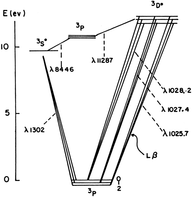
Figure 6. The energy level diagram of OI showing the possible fluorescence with L. Observable lines that are mostly affected are at 1302 and 8446. The process is most important in regions of large H optical depth.

Accurate treatment of line fluorescence requires a complete transfer calculation. There is also a local, less accurate solution, based on the escape probability method, that is simple to use and easy to incorporate into the statistical equilibrium equations. It involves the assumption of rectangular line profiles, (or more accurately a constant source function across the line profile), and gives quite good results. Its main disadvantage is the local treatment and the poor approximation at the line wings, where the source function is not constant.

Line fluorescence in AGNs has been a source of some confusion. Such processes are efficient in removing line photons from one transition, and pumping them into another, at frequencies where the radiation field is most intense, i.e. close enough to the line center for the source function to be constant. Further out into the line wings the source function is smaller and the pumping efficiency reduced. A separation of only a few Doppler widths between lines, can result in almost a zero fluorescence efficiency. This is the case even in very large optical depth lines, such as L, where the line profile is many Doppler widths wide.

Line photons can be destroyed by continuum absorption processes. This is sometimes called "continuum fluorescence" and is particularly important for optically thick lines, where the effective absorption optical depth is increased by the increased path length of the photons (see the k'() factor mentioned earlier). Important examples are the ionization of hydrogen n = 1 by resonance lines with < 912Å, the ionization of hydrogen from the n = 2 and n = 3 levels by L, MgII2798, H and FeII lines, and the ionization of neutral helium from the 2¹S and 2³P levels. Absorption by dust grains, that are mixed in with the gas, and by H^-, are other examples.

The escape probability method provides a simple local treatment for this situation. Consider again the two level atom, a line absorption cross sections of _l and a continuum absorption cross section, at the line frequency, _c. Define

(42)

and

(43)

The escape probability formalism suggests that in the presence of a continuum opacity source, an effective escape probability

(44)

is to replace ₂₁ in the statistical equilibrium equation (34). In this case, the emergent line flux, per unit volume, is

(45)

and the number of continuum absorptions (e.g. photoionizations) is

(46)

This treatment is local and does not take into account the absorption of line photons away from their point of creation. A possible way to improve it, in cases of large continuum optical depth, is to multiply Eqn. (45) by exp(-_c), where _c is a typical continuum optical depth, e.g. toward the inner surface of the cloud. The extra amount of continuum absorption should then be added to the expression in (46). This is not the only way to treat the continuum absorption process, and other, rather different methods, have also been suggested.

Absorption of external continuum radiation by spectral lines can be computed with the same formalism. Consider a point in the cloud where the optical depth to the illuminated surface, in a certain line, is _in. The probability of a photon emitted towards the continuum source to escape is (_in), which is also the probability of the external radiation to reach that point in the cloud. The local J (33) is thus increased by an amount corresponding to the unattenuated external flux multiplied by (_in). In the case of a central point source with luminosity L, the increase in J is

(47)

and the rate equation, omitting collisional and ionization processes, takes the form

(48)

where ₂₁ is the two-directional escape probability of equation (33). The process is important in cases of large ionization parameter. It can become significant in the partly neutral zone, where continuum absorption in spectral lines is immediately followed by collisional ionization from an excited state.

---

³ A component of microturbulence has been suggested to increase the line width and to reduce the optical depth. These are not considered here. We also do not consider velocity gradient (e.g. expansion) inside the clouds, that require a different escape probability function. Back.