


8.3. The Transfer Function
A more ambitious task is to try and map out the entire BLR, using information obtained from the light curves.
Given the assumption of linear response of the line to the continuum pulse,
we can formulate the relation between L(t) and E(t) using
a "transfer function",
 (t), (called also
a "response function"):
(t), (called also
a "response function"):
| (72) |
i.e. E(t) is the convolution of L(t) with
(t).
As can be seen from this equation,
(t), in
appropriate units, equals the
E(t) that would result from L(t) which is a
 -function at t =
0 (a continuum
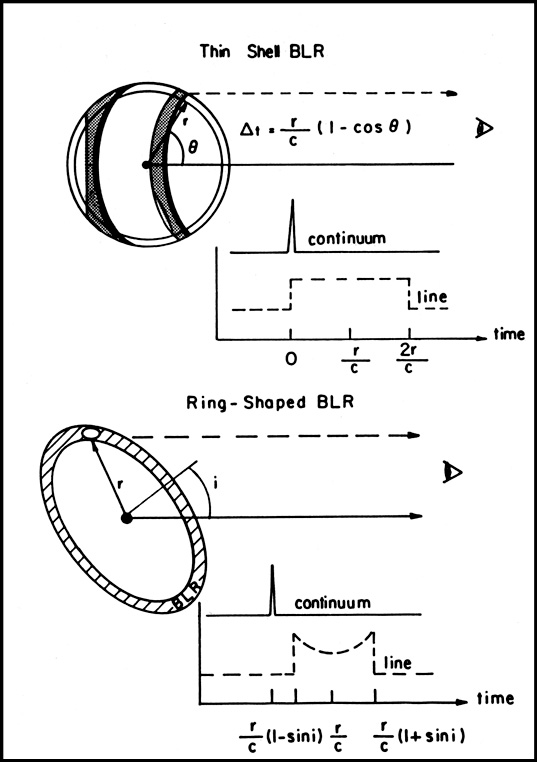
"flash"). For gas which is distributed in a thin shell of radius
r, the transfer
function is a "boxcar" shaped pulse, lasting from t = 0 until
t = 2r/c, with a
constant value of c / 2r. The rise at t = 0 is due
to the fact that the gas along
the line of sight appears to respond immediately to the continuum pulse, and
the information about the continuum and line variation arrived to the
observer simultaneously. The constant value of
(t) results from
the time delay of a
ring at a polar angle
-function at t =
0 (a continuum
"flash"). For gas which is distributed in a thin shell of radius
r, the transfer
function is a "boxcar" shaped pulse, lasting from t = 0 until
t = 2r/c, with a
constant value of c / 2r. The rise at t = 0 is due
to the fact that the gas along
the line of sight appears to respond immediately to the continuum pulse, and
the information about the continuum and line variation arrived to the
observer simultaneously. The constant value of
(t) results from
the time delay of a
ring at a polar angle  ,
r(1 - cos ) /
c, and the emissivity of the ring which is
proportional to its surface area. In a similar fashion the transfer
function of a
circular ring, inclined at an angle i to the line of sight, is
non-zero between times
r(1 - sini) / c to r(1 + sini) /
c, with its center at time r/c, This is illustrated in
Fig. 19.
,
r(1 - cos ) /
c, and the emissivity of the ring which is
proportional to its surface area. In a similar fashion the transfer
function of a
circular ring, inclined at an angle i to the line of sight, is
non-zero between times
r(1 - sini) / c to r(1 + sini) /
c, with its center at time r/c, This is illustrated in
Fig. 19.
|
Figure 19. The response of a thin shell and
an inclined ring emission line regions to a
|
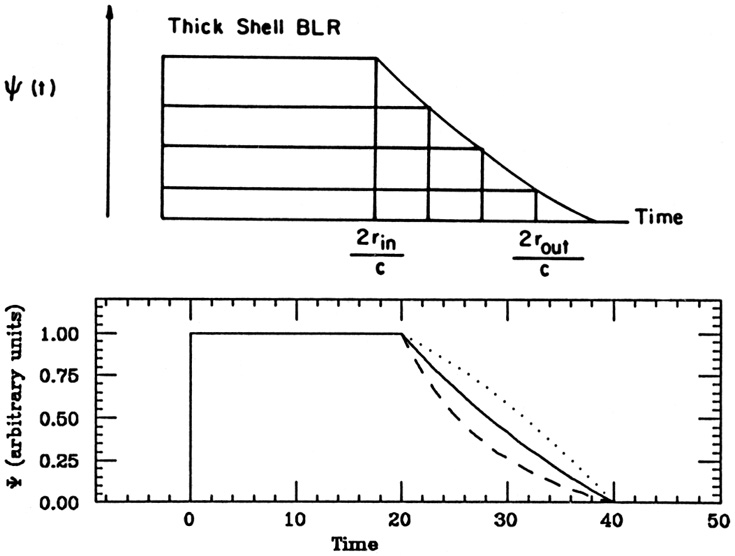
The transfer function of a thick shell is obtained by integrating the
thin shell
(t) over all
radii and weighting the contribution at each radius according to
the emissivity. The case of a shell of inner radius
rin and outer radius rout is
shown in Fig. 20. As seen from this diagram,
(t) is a constant
in time between
t = 0 and t = 2rin / c, and
declines to zero between t = 2rin / c
and t = 2rout / c.
The shape of the declining part depends on the gas distribution and
emissivity.
We can find this shape in the simple, optically thick case, using the
notation of
chapter 5 and the radial dependence of the
covering factor from equation (57),

| (73) |
This is illustrated in Fig. 20 for the cases of (p + q) = -2, 0 and +2. In a similar fashion, the transfer function of a thick disk is obtained from integrating over rings.
|
Figure 20. Bottom: Transfer functions of a
thick spherical shell of inner radius 10 time units
and outer radius 20 time units, for cases of (p + q) = -2 (dotted
line), 0 (solid line) and +2
(dashed line). The top half demonstrate the contributions of different
thin shells to
|
We see that valuable information about the gas distribution can be obtained
from (t) and it
is desirable to find this function and investigate its shape. In
principle, this is not a difficult task since
(t) can be
recovered from the data by applying the convolution theorem,
| (74) |
where ~ designates the Fourier transform. Performing this operation,
using the
observed L(t) and E(t) and transforming back to the time
domain, recovers
(t). In practice,
this is not a trivial task. E(t) and L(t) are often
unevenly sampled in time, have large gaps and span a relatively short
period. Under such
conditions, Fourier methods become problematic, and a meaningful transfer
function may become hard to obtain. Frequently sampled data, with a
sampling interval shorter than the typical variability time scale, can
be quite useful,
provided the light curve is long enough and the measurement error small
compared with the variability amplitude. There are improved statistical
methods
of recovering (t)
from the data (e.g. the maximum entropy method), using
additional constraints on its expected shape at different times.
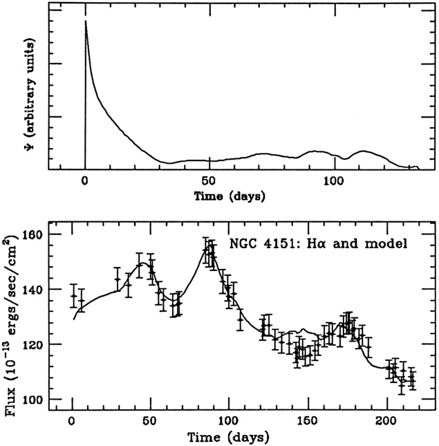
The transfer function for NGC 4151, obtained from applying the maximum
entropy method to the data presented here, is shown in
Fig. 21. The diagram
also shows the H light curve which is obtained by convolving this function
with the continuum light curve. The fit of the
H light curve is
quite satisfactory, suggesting that this
(t) is not a bad
approximation to the real transfer function. The empirical
(t) rises sharply
at t = 0 and drops to zero, in a
gradual way, over 30 days. This is consistent with a thick shell
geometry with a
very small inner radius and an outer radius of about 15 light-days. It
is also consistent with an edge-on disk (and other geometries) of similar
dimensions.
light curve which is obtained by convolving this function
with the continuum light curve. The fit of the
H light curve is
quite satisfactory, suggesting that this
(t) is not a bad
approximation to the real transfer function. The empirical
(t) rises sharply
at t = 0 and drops to zero, in a
gradual way, over 30 days. This is consistent with a thick shell
geometry with a
very small inner radius and an outer radius of about 15 light-days. It
is also consistent with an edge-on disk (and other geometries) of similar
dimensions.
|
Figure 21. Top: Transfer function for
NGC 4151, obtained from the line and continuum light
curves in Fig. 17, using a maximum
entropy deconvolution. Bottom: A model emission line
light curve obtained from the transfer function, on top of the
H |
A word of caution is in order. There are cases where several different transfer functions can fit the data equally well. This depends on the numerical method used and the quality of the light curves. For example, the features in the NGC 4151 transfer function at t ~ 50 - 100 days can be interpreted as due to some line emitting material far away from the nucleus. However, they can also be due to the numerical method used, given the freedom to put the emitting material anywhere around the central source. Physical constraints, such as an imposed upper limit on the BLR extension, should be used in such cases.
The experimental limitations are so severe that today the BLR transfer function is only known in one or two cases. The main problem in ground-based observations is the large amount of telescope time needed for proper sampling of the light curve, and the requirement of flux calibrated data. Space-born instrument are more suitable for the task but the aperture size of most of these is small and it has been extremely difficult to obtain enough observing time to perform the experiment. The first, complete ultraviolet data set was obtained in 1989 by a large group of IUE observers, who monitored the Seyfert 1 galaxy NGC 5548 for a continuous period of eight months. Much of our understanding of AGN variability is based on this data set.
The main theoretical limitation of the method is the assumption of
linearity. While the total line and diffuse continua emission of an
optically thick gas is
indeed proportional to the continuum flux, this is not case for
individual lines.
This is well illustrated in Fig. 8
that shows the response of different emission
lines to variations in the ionization parameter. The use of
(t) obtained for a
certain line to deduce the gas distribution must therefore be done with
great care. In addition, the geometry deduced from the empirical
transfer function
is not unique, and more information is required to choose among all possible
alternatives. Finally, all present day studies make the specific
assumption that
the observed optical, or ultraviolet continuum variations are
proportional to the
ionizing continuum variations. This is not necessarily the case and
alternatives
must also be investigated. Line profiles can provide additional
constrains on the gas distribution, as discussed in the next chapter.