5. Photoionization Models for a System of Clouds

Having calculated the emergent spectrum of isolated clouds, we now consider the gas distribution and the different ways to combine the emission from such clouds into a composite spectrum.

5.1. Spherical BLR Models

Consider a spherically symmetric system of clouds, extending from r_in to r_out. The mass of the individual clouds is conserved, but it is not necessarily the same for all clouds. The following physical parameters are all functions of r: the cloud number density n_c(r), the cloud particle density N, the cloud emissivity j_c(r), and the cloud velocity v(r).

Most cases of interest involve optically thick clouds, where energy conservation requires that the total emergent line and diffuse continuum luminosity equal the energy absorbed by the gas. In this case, the geometrical cross section of the cloud as seen from the center, A_c(r), is another useful parameter.

Designate _l(r) as the flux emitted by the cloud, in a certain emission line l, per unit projected surface area (erg s^-1 cm^-2), we have the following relation for the cloud emission:

(49)

We now make the following simplified assumptions about the radial dependence of the different parameters:

	(50)
	(51)
	(52)
	(53)

and

(54)

Using these definitions, the radial dependence of the ionization parameter is:

(55)

5.1.1. Covering factor. For optically thick clouds, it is useful to introduce the covering factor, C(r), which is the fraction of sky covered by photoionized gas clouds, as seen from the center. For a single cloud

(56)

and for a thin shell of thickness dr

(57)

The integrated covering factor can be estimated from the Lyman continuum observations (chapter 2) or from comparing the line and continuum luminosities (chapter 6). For the more luminous AGNs it is about 0.1 for the BLR and less than that for the NLR. It is thus justified to neglect obscuration and proceed on the assumption that the flux reaching the clouds depends only on r.

5.1.2. Integrated line fluxes. Given the calculated _l(r) for individual clouds (chapter 4), we can now integrate over r to obtain cumulative line fluxes. In the most general case

(58)

There are interesting cases where the number of radius dependent parameters is considerably reduced. An important example is a system of spherical clouds, of radius R_c(r), in pressure equilibrium with a confining medium of pressure P. The kinetic temperature of a photoionized gas is only a weak function of U, and we can safely assume that the radial dependences of P and N are identical ( r^-s). Since R³_c N = const., the cloud cross-section is

(59)

(i.e. s = -3/2q) and the column density is

(60)

Assume further that the clouds are moving in or out with their virial velocity. Mass conservation (n_cvr² = const.) requires that p = 2-t and substituting t = 1/2 we get the following radial dependence of the covering factor:

(61)

General considerations (chapter 9) suggest that 1 s 5/2 in many cases of interest. In particular, s = 9/4 corresponds to a case where the covering factor of a thin shell is proportional to the shell thickness.

The total flux, in all forms of emission, from a shell of thickness dr is proportional to dC(r) ⁽⁴⁾, and the cumulative flux is proportional to

(62)

This is, in fact, a good approximation for many individual lines (i.e. m = 2 is a good approximation for many lines).

We conclude that in those cases with s > 3/4, the cumulative covering factor, and therefore the integrated line emission, increases rapidly outward, and the innermost parts of the atmosphere do not contribute much to the line emission. For s 3/4 much of the line emission takes place close to the center and there is a natural boundary to the cloud distribution. Note, however, some potential difficulties. For example, the column density of ionized material depends on U and r, and clouds that are optically thick near r_out may become transparent closer in, or vice versa.

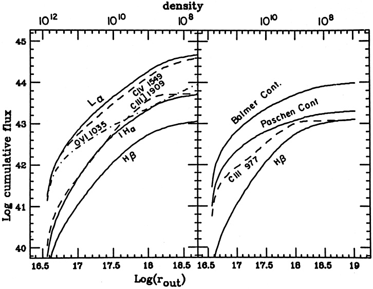
5.1.3. Specific models. Fig. 11 shows cumulative BLR line fluxes, as a function of r_out for a constant ionization parameter model, s = 2. They were calculated as explained in chapter 4, and added according to the prescription explained above. In this particular case, L(ionizing continuum) = 10⁴⁶ erg s^-1 U = 0.3 for all clouds and the normalization is such that N_col = 2 × 10²³ cm^-2 where N = 10¹⁰ cm^-3. The integration starts at r_in = 10^16.5 cm, where the density is 10¹² cm^-3, and carried out to large radii. Vertical cuts in the diagram correspond to a certain r_out and give the integrated line fluxes up to that radius.

Figure 11. Cumulative broad line fluxes, as a function of rout, for a model with U = 0.3 and s = 2. The model is calculated for the continuum shown in Fig. 7, assuming L(ionizing luminosity) = 1046 erg s-1. the value of rout for other luminosities is obtained by noting that rout L1/2.

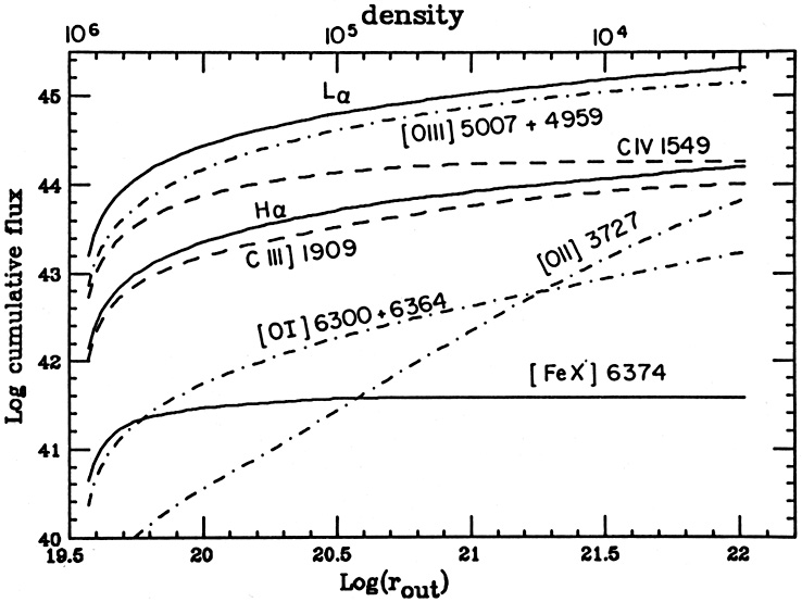
The narrow line fluxes can be integrated in a similar way, and Fig. 12 shows a model with s = 1, normalized such that U = 3.6 × 10^-2 where N = 10⁵ cm^-3 and N_col = 10²² cm^-2. Here again L(ionizing luminosity) = 10⁴⁶ erg s^-1, the inner radius is at 10^19.5 cm and the density there is 10⁶ cm^-3. Note that here, and in the BLR model of Fig. 11, the line intensity shown is normalized in such a way that the covering factor is unity at the outermost radius shown.

Figure 12. Cumulative narrow line fluxes, as a function of rout, for a model with s = 1 and parameters as explained in the text.

⁴ The radial dependence for individual lines is different, unless m = 2. Back.