9.4. Theoretical Line Profiles

9.4.1 Radial forces. We consider the general case of small clouds, moving through a confining medium. The radial motion of a cloud is determined by the gravitational acceleration, g_G, the radiative acceleration, g_rad, due to the absorption of the central continuum radiation, and the drag force, f_d. The equation of motion is:

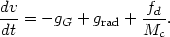
(82)

The radiation acceleration can be treated in a very general way by noting that the clouds are in ionization and thermal equilibrium. Energy conservation implies that the absorption of a photon of frequency is associated with cloud emission (all lines and diffuse continua) of h. The momentum transfer to the cloud, per unit time, is h / c. Thus, the radiative accelerating force is proportional to the total cloud emission. In the notation of chapter 5, the cloud emission is j_c(r), the mass of the cloud is M_c, and the radiative acceleration is proportional to j_c(r) / M_c.

We shall now be more specific about radiative acceleration. Consider first a fully ionized gas and assume, for simplicity, the pure hydrogen case. The mean energy of an ionizing photon is h and there are N_e² ionizations and recombinations per unit volume and time, each associated with a momentum transfer of h / c to the cloud. We neglect the absorption of non-ionizing continuum photons and line photons. The radiative acceleration is

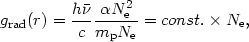
(83)

where m_p is the proton mass and we have neglected the temperature dependence of the recombination coefficient . Thus, theradiation acceleration of a fully ionized gas is proportional to the gas density and practically independent of the column density. (This is identical to the previous result since j_c(r) N_e² V_c and M_c N_e V_c, where V_c is the volume of the cloud.)

The other extreme situation is the case where all the ionizing flux is absorbed by an optically thick cloud. Here the amount of flux absorbed is proportional to the cloud cross section, A_c(r), and

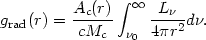
(84)

The properties of realistic clouds must be between these two cases. The ultraviolet radiation is absorbed in the fully ionized part and the harder radiation in the neutral zone. In particular, the cloud must be transparent at some frequency and the amount of momentum absorbed depends on the column density. It can be shown that the acceleration associated with the absorption of X-ray photons is proportional to 1/R²_c(1 + N_col / N₀), where N₀ 2 × 10²⁰ cm^-2.

Finally, the drag force exerted on a radially-moving cloud, depends on the cross-sectional area, the intercloud medium density and the relative velocity between the cloud and the intercloud medium.

Given a typical AGN continuum, we find, for optically thin gas,

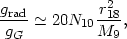
(85)

where r₁₈ = r / 10¹⁸cm and M₉ = M_BH / 10⁹ M. This ratio is larger than unity even for very large M_BH, and in the absence of strong drag forces, the radial motion of optically thin clouds is governed by outward radiation acceleration. As for optically thick clouds, g_rad / g_G depends on the density and column density of the clouds and must be calculated for the given situation.

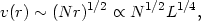
9.4.2 Pancake clouds. If clouds move radially through an intercloud medium, their shape and optical depth will be modified. Detailed calculations show that fully ionized, low mass clouds, approach a nearly spherical shape as they move out under the influence of radiation pressure acceleration. More massive clouds adopt a "pancake" shape, having much larger dimensions perpendicular to the direction of motion. This has important consequences to the emission line spectrum since relative line strength may depend on the cloud location. Moreover, not all clouds are accelerated outward and those that form closer in, where the ambient density is larger, may fall in under the influence of gravity. The net result is that the simple approximation adopted for A_c(r) in chapter 5 may not be valid in such cases. There are additional implications to the line profiles, as discussed below.

9.4.3 General line profiles. Consider a spherical system of isotropically emitting clouds, with a number density n_c(r) and emission per cloud j_c(r). We further assume that all of the cloud emission is represented by a single emission line. The wavelength dependence luminosity ("profile") in a line of rest wavelength ₀ is

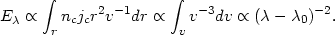
(86)

where µ = cos in a spherical coordinate system with its z axis parallel to the line of sight. Integration over the -function gives c/v ₀, provided 0 < | - ₀| c/₀ < 1.

We now make the simplifying assumptions of pure radial motion and a constant mass flow (mass conservation),

(87)

All clouds are assumed to form near r_in and experience a radial acceleration of g(r) = vdv/dr. Substituting into the line profile equation we get,

(88)

where v₁ is the largest of v(r_in) and | - ₀| c/₀. The line profile is logarithmic, E log(| - ₀|), in those cases where j_c / g(r)M_c is constant. Assuming mass conservation (87) this is equivalent to the following condition:

(89)

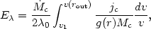
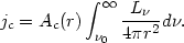
9.4.4 Line profiles for radiatively driven clouds. The general argument about the relation between the amount of radiation absorbed and the rate of momentum transfer (beginning of 9.4.1) suggests that in this case the radiative acceleration is proportional to j_c / M_c. Thus if the radiation pressure force is the dominant force, the line profile has a logarithmic shape. Below we demonstrate this for the two extreme cases considered earlier.

In the optically thin case, j_c V_c N_e², M_c N_e V_c and g_rad N_e. Thus j_c / g(r)M_c = const. and the line profile is logarithmic. In this case, the radial velocity at a distance where the density is N is approximately

(90)

where we have used the previously obtained radius-luminosity relation (75). With the estimate of g_rad / g_G (85), and the known density in the BLR, it can be shown that velocities of more than 10,000 km s^-1 can be obtained.

As for the optically thick case, the radiative acceleration is given by Eqn. (84) and the cloud emission by

(91)

Thus, j_c / g(r)M_c = const. and we recover the logarithmic line profile. Note again the assumption that all emission comes out in one emission line (or is divided among all lines in the same way at all distances) which is crucial for obtaining this particular line profile.

9.4.5 General logarithmic profiles. The conditions for a logarithmic line profile can be investigated in a more general way, using the radial dependences of the cloud parameters. Adopting Eqn. (89) as the basic requirement for a logarithmic shape, and the previous parametric descriptions, n_c(r) r^-p, A_c(r) r^-q and v(r) r^-t, we get the following requirement for a logarithmic line profile:

(92)

The line emissivity parameter, m, is approximately 2 for many emission lines, so an almost as general requirement is

(93)

As an example, consider infalling optically thick clouds, no radiation pressure and no drag force. Here t = 1/2 and mass conservation requires that 2 - p = t or p = 3/2. Logarithmic line profiles will result if q = 0 (also s = 0), i.e. constant radius clouds, In the two-phase scenario, this means a constant confining pressure throughout the emission line region.

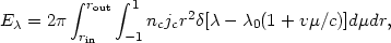
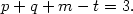
The s = 0 situation is illustrated below in more detail for a few velocity laws and complete photoionization models. The models are similar to the ones described in chapters 4 and 5, except that in this case the cumulative line fluxes are calculated with the assumption of a constant confining pressure and a constant gas density, s = 0. These integrated fluxes, as a function of r, are shown in Fig. 24.

Figure 24. Cumulative line fluxes, as a function of the outer radius, for a photoionization model with s = 0 (constant confining pressure) and N = 1010cm-3. The normalization of the model is such that U = 0.1 at Ncol = 1023.5 cm-2.

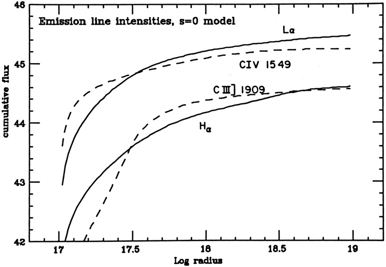
Line profiles for this cloud system have been calculated under several different assumptions. The first case is a decelerating outflow, with isotropic line emission and v r^-1/2. This velocity law satisfies the condition for a logarithmic profile (93) as is evident also from the L profile shown in Fig. 25. The profile is very similar to the CIV1549 profile shown in Fig. 23, except for the flat top, which is the result of the finite r_out used (i.e. no low velocity material). A flat-topped profile is a signature of radial flow motions with a weak v/r dependence and/or a small r_out / r_in. In the particular case shown here, the requirement for lines with smooth wings between 200 and 10,000 km s^-1, implies r_ont / r_in > 2500. This is an extreme and unrealistic ratio for the BLR.

Figure 25. L profiles obtained by integrating the line emission in the photoionization model of Fig. 24 with the velocity law indicated. Solid line: isotropic L line emission. Dashed line: anisotropic line emission (90% of the photons escape from the illuminated surface).

9.4.6 Orbital and chaotic motion. Chaotic (random orientation) cloud motion can produce line profiles that are in good agreement with some observations. Orbital motion can give good agreement too, at least for some emissivity laws. For example, it has been suggested that the BLR clouds are moving in parabolic orbits, with some net positive angular momentum. Reasonable assumptions about the distribution of clouds in angular momentum require that the cloud density be given by n_c(r) r^-1/2. Making the additional assumption of constant confining pressure (no change of the cloud cross section with r) we obtain j_c(r) r^-2 which, upon substituting into the line profile equation (86), gives:

(94)

Such profiles seem to fit nicely the far wings of many lines. Thus there is more than one dynamical model that can explain the observed profile.

As for the accretion disk model, in this case the motion is in a plane and a characteristic profile, made up of two humps and a central dip, results. The relative intensity of the profile components depends on the emissivity as a function of r and the size of the disk. Small disks would tend to give a large central dip, while in very large ones the dip is filled by emission from the outer, slowly rotating gas.

A few AGNs show disk-type line profiles and it has been suggested that this is a common phenomenon, except that the central dip in most other cases is filled in by emission from low velocity material, The distance of the low velocity material can be calculated, given the central mass. In some cases it is way beyond the outer boundary of the BLR, and may be inside the NLR. Such outer parts are well beyond the self gravity radius of a thin, radiation pressure supported accretion disk (chapters 5 and 10).

Much of the effort in fitting AGN line profiles by thin disk models has focused on the Balmer hydrogen lines in BLRGs. The specific disk models used are the ones discussed in chapter 5, where the low excitation lines are the result of back-scattering of the X-ray radiation onto the surface of the disk, at large radii. Such models predict little or no high ionization line radiation from the disk and it remains to be seen whether the observed L and CIV1549 lines are indeed different from the H and H line profiles in those objects.

9.4.7 Line asymmetry and wavelength shifts. All examples so far considered assume isotropic line emission. This is not necessarily the case for lines whose optical depth structure, within the cloud, is nonuniform. The most notable example is L, whose optical depth is very different in the ionized and neutral parts. Most of the emitted L photons escape through the illuminated cloud surface, and the radiation emitted in the outer direction is almost totally absorbed. Photoionization calculations predict that in a plane-parallel geometry, more than 95% of the broad L emission is emitted from the illuminated surface of the clouds. The effect is smaller, but not negligible, in other broad lines such as H, H and MgII2798.

Another example of anisotropic line emission is obscuration by dust. The intercloud medium may be dusty, causing line emission from the farther hemisphere to be fainter. Alternatively, the dust may be embedded in the clouds, mainly in the neutral part. The line emission from the back side of the clouds (the side away from the ionizing source), is weaker in this case. This is a likely situation in NLR clouds.

Anisotropic line emission has a direct consequence on the observed line profile of radially moving clouds. It introduces a profile asymmetry whose magnitude depends on the degree of anisotropy and the velocity pattern. For example, in outflow motion the L profile would show a strong red asymmetry (red wing stronger than blue wing). A similar asymmetry is obtained for outflowing dusty clouds, whose dust particles reside in the back of the clouds. An outflow motion through a dusty intercloud medium gives a blue asymmetry. Fig. 25 shows the broad L profile resulting from the outflowing s = 0 atmosphere, when the L anisotropy is taken into account. The strong red asymmetry is clearly visible in this case.

Asymmetric broad line profiles are indeed observed in some cases, but in many AGNs the line profiles, including L, are quite symmetric. There are several possible explanations for this. The first and most obvious one is that there is little, if any, radial motion of BLR clouds. There are other evidences (section 9.5) to support this claim. Alternatively, some of the L emission may originate in outflowing (or infalling) optically thin clouds, whose emission pattern is much more isotropic. The obvious difficulty is the presence of strong, low excitation lines, that require large neutral hydrogen column densities. Pancake shaped clouds have a variable column density, and may be thin along their rim. This helps to reduce the profile asymmetry in a radially moving system.

An alternative explanation for symmetric line profiles in a radially moving system is the presence of some scattering material in the vicinity of the clouds. The scatterers may be the hot electrons in the HIM or dust particles in the NLR. The main cause of asymmetry is the weak flux from the hemisphere nearer to the observer and there are several ways by which this can change in the presence of scatterers. First, the scattered ionizing radiation can hit the back, neutral side of the clouds, producing more ionization and line emission. Second, if the intercloud medium is optically thick, the radiation observed from the farther hemisphere is reduced. Third, the inward emitted line photons in the near hemisphere can be scattered back into the line of sight. Fig. 26 shows two L profiles, resulting from the same cloud system as before, but moving in this case through a Compton thick HIM. The line profiles are calculated for the cases of _es = 0 and _es = 2, and the latter is indeed more symmetric.

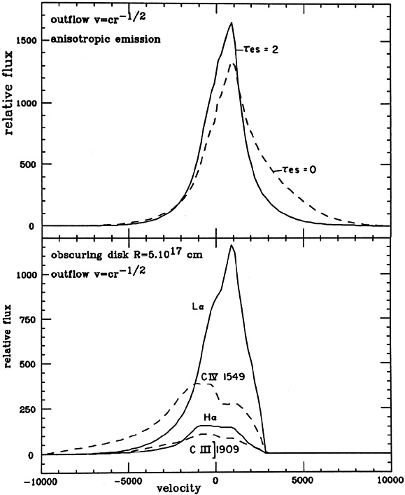
Figure 26. Top: Unnormalized L profiles for the s = 0 outflowing atmosphere, showing the effect of a Compton thick medium. The L emission from the clouds is highly anisotropic but the line asymmetry is reduced, compared to the Compton thin case, due to scattering related effects. Bottom: The same, model, with es = 0, combined with a central obscuring disk of radius 5 × 1017 cm. Note the wavelength shift of the line centers.

The wavelength shift of some broad lines in high luminosity AGNs is definitely of great significance. In the time of writing there is no satisfactory explanation for this. One idea is that the shift is caused by a combination of obscuration and outflow motion. Consider for example a decelerating outflow around a large accretion disk, with U decreasing outward. The high excitation lines, like CIV1549, are formed near the disk and much of their red-wing (emission from the other side of the disk) is not observed. Lower excitation lines, such as MgII2798, are produced further away from the disk, where the obscuration is smaller. Their central wavelength is closest to the "true" redshift. An illustration is shown in Fig. 26. This is the same s = 0 outflow model as before but this time with a central obscuring disk of radius 5 × 10¹⁷ cm. Some wavelength shift between L, CIV1549 and H, is indeed observed, but all lines are asymmetric and the velocity difference is small. A more complex situation, of outflow combined with a flat rotating system whose low ionization lines are predominately from material in the plane of the disk, may give a better match to the observations.