


2.7. Spatial distribution of galaxies
The most regular clusters show a smooth galaxy distribution with a
concentrated
core (Figure 4;
Table 1). In general, models to
describe the galaxy distribution in
these clusters will possess at least five parameters, which can be taken
to be the
position of the cluster center on the sky, the central projected density
of galaxies per unit area of the sky
 0, and
two distance scales rc and Rh. The
core radius rc
is a measure of the size of the central core, and is usually defined so
that the projected galaxy density at a distance rc
from the cluster center is one half of the central density
0. The
halo radius Rh measures the maximum radial extent of
the cluster. Of course, the observed value of the central density
0 must
depend on the range of galaxy magnitudes observed, and the values of
other parameters may also depend on galaxy magnitude. If the cluster
is elongated, at least two more parameters are necessary; these can be
taken to be the orientation of the semimajor axis of the cluster on the
sky, and the ratio of semimajor to semiminor axes. However, spherically
symmetric galaxy distributions will be discussed first, and
rc and Rh will be
assumed to be independent of galaxy mass or luminosity. Then, one can
write
0, and
two distance scales rc and Rh. The
core radius rc
is a measure of the size of the central core, and is usually defined so
that the projected galaxy density at a distance rc
from the cluster center is one half of the central density
0. The
halo radius Rh measures the maximum radial extent of
the cluster. Of course, the observed value of the central density
0 must
depend on the range of galaxy magnitudes observed, and the values of
other parameters may also depend on galaxy magnitude. If the cluster
is elongated, at least two more parameters are necessary; these can be
taken to be the orientation of the semimajor axis of the cluster on the
sky, and the ratio of semimajor to semiminor axes. However, spherically
symmetric galaxy distributions will be discussed first, and
rc and Rh will be
assumed to be independent of galaxy mass or luminosity. Then, one can
write
| (2.6) |
where n(r) is the spatial volume density of galaxies at a
distance r from the cluster center, n0 is the
central (r = 0) density,
(b) is the
projected surface density at a projected radius b, and f and F
are two dimensionless functions. Obviously,
| (2.7) |
A number of models have been proposed to fit the distribution of galaxies. Among the simplest are the isothermal models, which assume a Gaussian radial velocity distribution for galaxies (equation 2.5). If one further assumes that the velocity distribution is isotropic and independent of position, that the galaxy distribution is stationary, and that galaxy positions are uncorrelated, then one can write the galaxy phase space density f(r, v) as
| (2.8) |
Now, the time-scale for two-body gravitational interactions in a cluster is
much longer than the time for a galaxy to cross the cluster (see
Section 2.9).
Thus the galaxies can be considered to be a collisionless gas, and the
phase space density f is conserved along particle trajectories
(Liouville's theorem); f is then a
function of only the integrals of the motion ('Jeans' theorem'). If the
velocity distribution is isotropic, f does not depend on the
orbital angular momentum of
the galaxies, and can only depend on the energy per unit mass
 = 1/2
v2 +
= 1/2
v2 +
 (r),
where (r) is the
gravitational potential of the cluster. If we measure
(r) relative to the
cluster center, the galaxy spatial distribution is thus
n(r) = n0
exp[-(r) /
r2].
If the mass in the cluster is distributed in the same
way as the galaxies, then Poisson's equation for the gravitational potential
becomes
(r),
where (r) is the
gravitational potential of the cluster. If we measure
(r) relative to the
cluster center, the galaxy spatial distribution is thus
n(r) = n0
exp[-(r) /
r2].
If the mass in the cluster is distributed in the same
way as the galaxies, then Poisson's equation for the gravitational potential
becomes
| (2.9) |
where m is the mass per galaxy
(Chandrasekhar, 1942).
It is conventional to make the change of variables

 /
r2,
/
r2,
 r /
r /  ,
r /
(4
,
r /
(4 Gn0
m)1/2. Then
the equation for is
Gn0
m)1/2. Then
the equation for is
| (2.10) |
subject to the boundary conditions (assuming the density is regular at the
cluster center) of = 0,
d /
d = 0 at
= 0. Equation
(2.10) is identical to the
equation for an isothermal gas sphere in hydrostatic equilibrium
(Chandrasekhar, 1939).
|
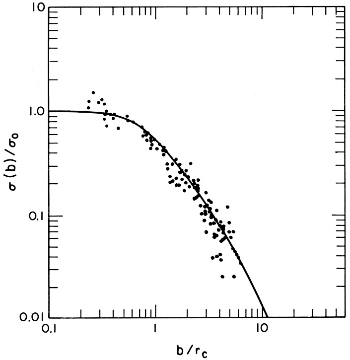
Figure 4. The dots give the projected
galaxy number density observed in 12 regular clusters, from
Bahcall (1975).
The observed number densities are
normalized to the central surface number density
|
The galaxy density distribution in this isothermal sphere model is then
n() =
n0
exp[-()].
The projected galaxy density can be calculated from
equation (2.7) and written as
(b) =
0
Fisot(b /
). For
convenience, the
core radius rc is defined as rc
3, because
Fisot(3)
 0.502, which is
obviously close to one-half. The central volume density and projected
density are related by
0
6.06n0 = 2.02n0
rc. Unfortunately, neither
()
nor Fisot can be represented by simple analytic
functions. Relatively
inaccurate tables of these functions are given in Zwicky (1957, p. 139),
and more accurate economized analytic approximations to
and Fisot
have been given by
Flannery and Krook
(1978),
and Sarazin (1980),
respectively.
0.502, which is
obviously close to one-half. The central volume density and projected
density are related by
0
6.06n0 = 2.02n0
rc. Unfortunately, neither
()
nor Fisot can be represented by simple analytic
functions. Relatively
inaccurate tables of these functions are given in Zwicky (1957, p. 139),
and more accurate economized analytic approximations to
and Fisot
have been given by
Flannery and Krook
(1978),
and Sarazin (1980),
respectively.
At large radii
>> 1,
n()
2n0
/ 2,
and the total number of galaxies and
total mass diverge in proportion to r. Thus the isothermal sphere
cannot
accurately represent the outer regions of a finite cluster. A number of
methods to truncate the isothermal distribution have been used. If one is
primarily concerned with representing the galaxy distribution near the core,
and if one is not concerned with determining dynamically consistent
velocity and spatial distributions, one can simply truncate the isothermal
distribution at some radius.
Zwicky (1957,
p. 140) and
Bahcall (1973a)
have truncated the isothermal distribution with a uniform surface
density cutoff C:
| (2.11) |
The cluster galaxy density then falls to zero at a radius
Rh given by Fisot(Rh,
) =
C / 6.06.
Bahcall (1973a)
also defines a modified central surface density parameter
 0 /(6.06 -
c); then, for small C<<
2,
the central volume density is just n0
0[1 -
(C / 2)2]
/ (6.06)
/
.
The solid curve for the surface density in
Figure 4 is given by equation 2.11.
0 /(6.06 -
c); then, for small C<<
2,
the central volume density is just n0
0[1 -
(C / 2)2]
/ (6.06)
/
.
The solid curve for the surface density in
Figure 4 is given by equation 2.11.
King (1966) has developed self-consistent truncated density distributions for clusters. The phase-space density he assumes is
| (2.12) |
where r is the radial velocity
dispersion in an untruncated cluster. The
velocity distribution is thus truncated at the escape velocity
ve: f(r, |v|
is the radial velocity
dispersion in an untruncated cluster. The
velocity distribution is thus truncated at the escape velocity
ve: f(r, |v|
 ve) = 0
where ve2 =
-2(r), and the
potential goes to zero at infinity
() = 0. King
showed that equation (2.12) gave an approximate solution to the
Fokker-Planck equation for a finite cluster subject to two-body
gravitational encounters. As shown in
Section 2.9, galaxy clusters are
nearly collisionless; however, it is
possible that equation (2.12) is a reasonable approximation for the
truncated phase-space density. The phase-space density f in
equation (2.12) is a function of only the energy per unit mass
and the parameter
r2, and thus
satisfies
Jeans' theorem. King integrates equation (2.12) over all velocities to
give the density n(r) as a function of the potential
(r), and then solves
Poisson's equation to give a self-consistent potential. The
density n(r) in
these models falls continuously to zero at a finite radius
Rh. The models
can be scaled in distance and central density as with the unbounded
isothermal models described earlier. The only characteristic parameter is
r(0) /
r or equivalently
Rh / rc (where rc
is again the core radius). King
prefers to use the potential difference between cluster center and edge,
W0
[(Rh) -
(0)] /
r2. These
models predict that the velocity dispersion
declines in the outer portions of the cluster, as is observed in
Coma
(Rood et al.,
1972).
ve) = 0
where ve2 =
-2(r), and the
potential goes to zero at infinity
() = 0. King
showed that equation (2.12) gave an approximate solution to the
Fokker-Planck equation for a finite cluster subject to two-body
gravitational encounters. As shown in
Section 2.9, galaxy clusters are
nearly collisionless; however, it is
possible that equation (2.12) is a reasonable approximation for the
truncated phase-space density. The phase-space density f in
equation (2.12) is a function of only the energy per unit mass
and the parameter
r2, and thus
satisfies
Jeans' theorem. King integrates equation (2.12) over all velocities to
give the density n(r) as a function of the potential
(r), and then solves
Poisson's equation to give a self-consistent potential. The
density n(r) in
these models falls continuously to zero at a finite radius
Rh. The models
can be scaled in distance and central density as with the unbounded
isothermal models described earlier. The only characteristic parameter is
r(0) /
r or equivalently
Rh / rc (where rc
is again the core radius). King
prefers to use the potential difference between cluster center and edge,
W0
[(Rh) -
(0)] /
r2. These
models predict that the velocity dispersion
declines in the outer portions of the cluster, as is observed in
Coma
(Rood et al.,
1972).
Unfortunately, none of these bounded or unbounded isothermal models can be represented exactly in terms of simple analytic functions. However, King (1962) showed that the following analytic functions were a reasonable approximation to the inner portions of an isothermal function:
| (2.13) |
where 0 =
2n0rc. At large radii r >>
rc, n(r)
n0(rc / r)3 in the
analytic King
model; thus the cluster mass and galaxy number diverge as ln(r /
rc). Although
this is a slower divergence than the unbounded isothermal model, this
analytic King model also must be truncated at some finite radius
Rh.
Another analytic model is that of de Vaucouleurs (1948a), which was proposed to fit the distribution of surface brightness in elliptical galaxies. However, this distribution also fits many regular clusters (de Vaucouleurs, 1948b). The projected density is
| (2.14) |
where re is an effective radius such that one half of
the galaxies lie at
projected radii b  re. Accurate tables of the three-dimensional density and
potential for this model have been given by
Young (1976).
The de Vaucouleurs
form has several advantages over the isothermal function. It has only one
distance scale, the effective radius re. It also
converges to a finite total number of
galaxies and cluster mass without a cutoff radius. Numerical simulations
of the
collapse of clusters seem to lead to distributions similar to this form
(see Section 2.9.2).
Unfortunately, the de Vaucouleurs form has not been
widely used to fit galaxy distributions in clusters, and there have been
few attempts to determine
objectively whether it or the isothermal models give better fits to the
actual distributions.
re. Accurate tables of the three-dimensional density and
potential for this model have been given by
Young (1976).
The de Vaucouleurs
form has several advantages over the isothermal function. It has only one
distance scale, the effective radius re. It also
converges to a finite total number of
galaxies and cluster mass without a cutoff radius. Numerical simulations
of the
collapse of clusters seem to lead to distributions similar to this form
(see Section 2.9.2).
Unfortunately, the de Vaucouleurs form has not been
widely used to fit galaxy distributions in clusters, and there have been
few attempts to determine
objectively whether it or the isothermal models give better fits to the
actual distributions.
One major difference between the isothermal functions and the de
Vaucouleurs law is that the latter has a density cusp at the cluster
center; in fact,
as can be seen from Figure 4, many clusters show
these cusps, which much be
removed in order to fit isothermal sphere models to the galaxy
distributions.
Beers and Tonry (1986)
show that the galaxy distribution in clusters
is very sensitive to the position chosen for the cluster center, and that
many clusters have central number density spikes if the cluster center is
assumed to correspond to the position of a cD galaxy
(Section 2.10.1) or the
maximum of the X-ray surface brightness
(Section 4.4.1). They find that
the surface density near this cusp varies roughly as
(b)
 b-1, which
is consistent with a singular isothermal sphere (one with
rc
b-1, which
is consistent with a singular isothermal sphere (one with
rc
 0), or
with an anisotropic galaxy velocity distribution, with an excess of radial
orbits. The presence of these cusps is important to understanding the
occurrence of multiple nuclei and companions about cD galaxies
(Section 2.10.1).
0), or
with an anisotropic galaxy velocity distribution, with an excess of radial
orbits. The presence of these cusps is important to understanding the
occurrence of multiple nuclei and companions about cD galaxies
(Section 2.10.1).
Another useful fitting form is the Hubble (1930) profile, which is sometimes used to fit the light distribution in elliptical galaxies. It is
| (2.15) |
which has the same asymptotic distribution as equation (2.13).
These models (equations 2.11-2.15) have been used to fit the projected distribution of galaxies. In most cases, the galaxy distributions have been fit to the truncated isothermal model (equation 2.11). Figure 4 shows the surface number density distributions in 15 regular clusters, from Bahcall (1975), along with the fitting function (equation 2.11). A compilation of the values of the core radii which have been derived for clusters is given in Table III of Sarazin (1986a), which includes values from Abell (1977), Austin and Peach (1974a), Bahcall (1973a, 1974a, 1975), Bahcall and Sargent (1977), Birkinshaw (1979), Bruzual and Spinrad (1978a, b), des Forets et al. (1984), Dressler (1978c), Havlen and Quintana (1978), Johnston et al. (1981), Koo (1981), Materne et al. (1982), Quintana (1979), Sarazin (1980), Sarazin and Quintana (1987), and Zwicky (1957).
Bahcall (1975) has suggested that the core radii of regular clusters are all very similar, with an average value
| (2.16) |
Sarazin and Quintana (1987) find that this may be true for the most compact, regular clusters. However, they also find that the core radius and galaxy distribution depend on the morphology of the cluster (Section 2.5).
The statistical uncertainty in the determination of the core radius or
central density of a cluster tends to be rather large
( 30%), because
even in a rich cluster only a small fraction of the galaxies are within
the core. However, the errors in
0 and
rc are highly anticorrelated, so that the product
(0rc)
is relatively well-determined. The reason for
this is that the number of galaxies within a projected radius b
such that
rc < b << Rh is
roughly N(b)
2.17(0rc)b for an isothermal
model. Thus the uncertainty in the product
(0rc)
tends to be determined by Poisson
statistics on the total number of cluster galaxies observed, and not just by
the smaller number in the core
(Sarazin and Quintana,
1987).
Bahcall (1977b,
1981)
has defined a related quantity
30%), because
even in a rich cluster only a small fraction of the galaxies are within
the core. However, the errors in
0 and
rc are highly anticorrelated, so that the product
(0rc)
is relatively well-determined. The reason for
this is that the number of galaxies within a projected radius b
such that
rc < b << Rh is
roughly N(b)
2.17(0rc)b for an isothermal
model. Thus the uncertainty in the product
(0rc)
tends to be determined by Poisson
statistics on the total number of cluster galaxies observed, and not just by
the smaller number in the core
(Sarazin and Quintana,
1987).
Bahcall (1977b,
1981)
has defined a related quantity
 0 as the
number of 'bright
galaxies' with projected positions within 0.5 Mpc of the cluster
center. Here,
bright galaxies are those no more than two magnitudes fainter than the
third brightest galaxy (m
m3 +
2). Of course, the magnitude of the
third brightest galaxy m3 itself depends on richness;
0 is the number
corrected for richness assuming a universal luminosity function
(Section 2.4).
From the discussion above, it is clear that
0
(0rc),
if 0 is taken
at a standard luminosity level (for example,
L*
(Section 2.4)), and if
rc
0 as the
number of 'bright
galaxies' with projected positions within 0.5 Mpc of the cluster
center. Here,
bright galaxies are those no more than two magnitudes fainter than the
third brightest galaxy (m
m3 +
2). Of course, the magnitude of the
third brightest galaxy m3 itself depends on richness;
0 is the number
corrected for richness assuming a universal luminosity function
(Section 2.4).
From the discussion above, it is clear that
0
(0rc),
if 0 is taken
at a standard luminosity level (for example,
L*
(Section 2.4)), and if
rc
 0.5 Mpc <<
Rh.
0.5 Mpc <<
Rh.
Because they are better determined statistically than the core radius
rc or center surface density
0,
(0rc)
and 0 are
often more useful as richness
parameters when searching for correlations of integral properties of
clusters in the
optical, radio, and X-ray region. However, when comparing detailed spatial
distributions the core radius is needed.
For example, from the arguments given above
0rc
0
n0 rc2, if
0
and n0 are taken at a standard luminosity level.
From equation (2.9), rc2 =
9r2
/ 4
Gn0m, where m is the average galaxy mass
m
 0
/ n0, and
0 is
the central mass density. As n0 is defined at a fixed
luminosity level, this gives
(0
rc)
0
(M/L)-1
r2,
where (M/L) is the mass-to-light ratio of
the cluster (Section 2.8).
Bahcall (1981)
finds the empirical correlation
0
21(r
/103 km/s)2.2, which suggests that cluster
mass-to-light ratios decrease with
r. This
relationship may be useful for
providing quick estimates of the velocity dispersions of clusters.
0
/ n0, and
0 is
the central mass density. As n0 is defined at a fixed
luminosity level, this gives
(0
rc)
0
(M/L)-1
r2,
where (M/L) is the mass-to-light ratio of
the cluster (Section 2.8).
Bahcall (1981)
finds the empirical correlation
0
21(r
/103 km/s)2.2, which suggests that cluster
mass-to-light ratios decrease with
r. This
relationship may be useful for
providing quick estimates of the velocity dispersions of clusters.
Several other size scales can be determined for clusters. The halo
radius Rh
gives the outermost limit of the cluster. Unfortunately, this is very poorly
determined, because it depends critically on the assumed background.
Moreover, clusters often have very extended haloes or are embedded in
extended regions of enhanced density (superclusters). For Coma, the main
isothermal distribution of galaxies extends to roughly
4h50-1 Mpc;
there is then a low-density halo extending to
10h50-1 Mpc, which
blends into the Coma supercluster which extends to a radius of about
35h50-1 Mpc
(Rood et al.,
1972;
Rood, 1975;
Chincarini and Rood,
1976;
Abell, 1977;
Gregory and Thompson,
1978;
Shectman, 1982).
However, studies of the galaxy covariance function
(Peebles, 1974)
suggest that
there are no preferred scales for galaxy clustering and that the outer
regions of clusters and superclusters represent a continuous distribution of
clustering.
Other size scales for clusters have been measured that are intermediate between the core and halo size; they include the harmonic mean galaxy separation (Hickson, 1977), which is related to the gravitational radius RG of a cluster (Section 2.8), the de Vaucouleurs effective radius re defined by equation (2.14), the mean projected distance from the cluster center (Noonan, 1974; Capelato et al., 1980), and the Leir and van den Bergh radius (1977).
While the distribution functions for galaxies discussed above are
spherically symmetric, most clusters appear to be at least slightly
elongated, and some are highly elongated
(Sastry, 1968;
Rood and Sastry, 1972;
Rood et al.,
1972;
Bahcall, 1974a;
MacGillivray et
al., 1976;
Thompson and Gregory,
1978;
Carter and Metcalfe,
1980;
Dressler, 1981;
Binggeli, 1982).
Carter and Metcalfe
(1980)
and Binggeli (1982)
give ellipticities and position angles for samples of Abell
clusters. Their results suggest that clusters have average intrinsic
ellipticities of
0.5 - 0.7; thus
clusters are actually much more elongated on average than
elliptical galaxies.
Carter and Metcalfe (1980) and Binggeli (1982) find that the position angles for the long axes of clusters are significantly aligned with the axis of the first-brightest cluster galaxy. In Sections 2.9.3 and 2.10.1, it is shown that such alignments may result if the first-brightest galaxies are produced by the merger of smaller galaxies through dynamical friction. They might also be produced during the collapse of the cluster.
Thompson (1976) has suggested that the axes of many of the elliptical galaxies in clusters may be aligned with the cluster axis; Adams et al. (1980) find a similar effect in two linear (L; see Section 2.5) clusters. Helou and Salpeter (1982) and Salpeter and Dickey (1985) do not find such alignments for the axes of spiral galaxies in the Virgo or Hercules clusters.
Binggeli (1982)
finds that the long axes of Abell clusters tend to
point at one another, even when the clusters are separated by as much
as
30h50-1 Mpc. The alignments of nearby
clusters were found to show evidence of a correlation even up to
distances a factor of three larger.
In the previous discussion, it has been assumed that the galaxy density decreases monotonically with distance from the cluster center. However, Oemler (1974) found a plateau or local minimum in the projected distribution of galaxies in many clusters at a radius of about 0.4RG (where RG is the gravitational radius). These features would imply the existence of significant oscillations in the three-dimensional galaxy density, although the process of deprojecting to counts is rather unstable (Press, 1976). Although these features are not statistically very significant in any one case, they do appear in a large number of clusters (Omer et al., 1965; Bahcall, 1971; Austin and Peach, 1974a).