5.1. Sky Maps of VELMOD Residuals

VELMOD does not assign galaxies a unique distance (Section 2.2.1). Thus, there is no unique measure of the amount by which their observed and predicted peculiar velocities differ. However, there is a well-defined, expected apparent magnitude for each object,

(21)

where P(m|, cz) is given by equation (11). Similarly, the rms dispersion about this expected value is

(22)

Note that m is not equal to the TF scatter; it also includes the combined effects of velocity noise, peculiar velocity gradients, and density changes along the line of sight. At large distances, m tends toward _TF (although dispersion bias can make it smaller; cf. Willick 1994). With the above definitions, one can define a normalized magnitude residual for each galaxy,

(23)

The normalized residual has the virtue of having unit variance for all objects. In contrast, the variance of the unnormalized magnitude residual m - E(m, cz) depends on distance (velocity noise is more important for nearby objects), while the variance of a peculiar velocity residual formed from the magnitude residual (eq. [24]) grows with distance. The normalized magnitude residual _m is a measure of the correctness of the IRAS velocity model. If, in a given region, _m > 0 in the mean, galaxies in that part of space must be more distant than IRAS predicts them to be, i.e., they have negative radial peculiar velocity relative to the IRAS prediction. Regions in which _m < 0 in the mean have positive radial peculiar velocities relative to IRAS.

We will use the normalized magnitude residual below in our quantitative analysis of residuals, but let us first visualize this residual field on the sky, by converting _m into the corresponding radial peculiar velocity residual u. If we were to do this for each galaxy individually, the ~ 20% distance errors due to TF scatter would completely hide the systematic departures from the IRAS model. Instead, we will compute smoothed velocity residuals. This procedure is the most well behaved if we first smooth _m and then convert the result into u. We first place each galaxy at the distance d assigned it ⁽¹³⁾ by the IRAS velocity model; this is a redshift-space distance, so our calculation is unaffected by Malmquist bias. Then, for each galaxy i, we compute a smoothed residual _m,i^s as the weighted sum of the residuals _m of itself and its neighbors j, where the weights are w_ij = exp (-d_ij² / 2S_i²), and d_ij is the IRAS-predicted distance between galaxies i and j. We take the smoothing length S_i to be S_i = d_i / 5. The smoothed residual _m,i^s is converted into a smoothed velocity residual according to

(24)

where m_i is given by equation (22). The quantity f_i is given by exp (-_i² / 2), where _i = 0.46 m_i / (_j w_ij)^1/2; it guarantees that u_i^s, which is lognormally distributed, has an expectation value of zero if m_i (which is normally distributed) does also (cf. Willick 1991, Section 6.3, for details).

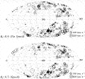
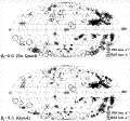
In Figures 10, 11, and 12, we plot VELMOD velocity residuals on the sky for the redshift ranges 0-1000 km s^-1, 1000-2000 km s^-1, and 2000-3000 km s^-1, respectively. In each figure, the top panel shows residuals from the _I = 0.6 (no-quadrupole) fit, and the bottom panel shows residuals from the _I = 0.5 (quadrupole-modeled) fit, the VELMOD runs closest to the maximum likelihood value of _I for each case. The plots reveal why the addition of the quadrupole results in a large increase of likelihood. In each redshift range, the no-quadrupole fits show coherent negative velocity residuals both in the Ursa Major region (l 150°, b 65°) and at b -60°, l 30°, and l 330°. In both of these regions, the addition of the quadrupole reduces the amplitude of the residuals significantly. In other parts of the sky, smaller but still significant coherent residuals are reduced with the addition of the quadrupole. This shows that the pattern of departure from the pure IRAS velocity field is well modeled by a quadrupolar flow of modest amplitude and therefore has the simple physical interpretation we discussed in Section 4.4.

Figure 10. VELMOD velocity residuals plotted on the sky in Galactic coordinates, for objects with 0 < czLG 1000 km s-1. The top panel is for the I = 0.6 run without the quadrupole. The bottom panel is for the I = 0.5 run with the quadrupole modeled. The open circles indicate objects that are inflowing relative to the IRAS prediction; the stars indicate outflowing objects.

Figure 11. Same as Fig. 10, but for objects with 1000 < czLG 2000 km s-1.

Figure 12. Same as Fig. 10, but for objects with 2000 < czLG 3000 km s-1.

In the bottom panels, it is difficult to find any well-sampled region within 2000 km s^-1 where u 100 km s^-1. This is all the more remarkable because the TF errors themselves are of order 300 km s^-1 per galaxy at a distance of 1500 km s^-1. Figure 12 does show several high-amplitude residuals. However, at 2500 km s^-1, the TF residual for a single object is 500 km s^-1, so when the effective number of galaxies per smoothing length is only a few, velocity residuals of several hundred km s^-1 are expected from TF scatter only. In well-sampled regions, one sees that in general u 150 km s^-1, the only exception being a patch of large ( 250 km s^-1) positive residuals at l 330°, b -20°. In the b > 0° part of the Great Attractor region at l 300°, the residuals are less than 100 km s^-1, even in this highest redshift shell. This is significant, given the often heard claims that the IRAS model cannot fit the observed flow into the Great Attractor. Although some residual coherence is apparent, we will demonstrate in Section 5.2 that this is largely because of the smoothing.

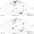
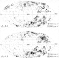
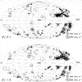
In Figures 13, 14, and 15, we again plot VELMOD residuals on the sky for the three redshift ranges, now for the two values of _I most strongly disfavored by the likelihood statistic in the range studied, _I = 0.1 (top panels) and _I = 1.0 (bottom panels). In each plot, the quadrupole of Figure 4 has been included. These plots, which should be compared with the bottom panels of Figures 10, 11, and 12, demonstrate why very low and high _I do not fit the TF data well. In each redshift range, these models exhibit large coherent residuals. For _I = 0.1, we see large negative peculiar velocities relative to IRAS in the Ursa Major region at cz 2000 km s^-1. Indeed, the residual plot for _I = 0.1 (with quadrupole included) shows many of the same features as the no-quadrupole model with _I = 0.6, because the IRAS field itself contributes some of the needed quadrupole. However, the IRAS contribution scales with _I and is thus inadequate at low _I. At _I = 1.0, many of the systematic residuals associated with the quadrupole are gone, especially in Ursa Major. However, other regions show highly significant residuals: at l 150°, b -20°, and cz 1000 km s^-1, for example, one sees negative peculiar velocity residuals of amplitude 200 km s^-1, which is significant at such small distances. In the same redshift range, at l = 270°-360°, b < 0°, there are positive velocity residuals of amplitude 150 km s^-1. These regions exhibit much smaller residuals in the _I = 0.5 model.

Figure 13. Same as Fig. 10, except now the results for I = 0.1 and I = 1.0 are shown. In each case, the quadrupole is the same as it was for the best-fit model (I = 0.5).

Figure 14. Same as Fig. 13, but for objects with 1000 < czLG 2000 km s-1.

Figure 15. Same as Fig. 14, but for objects with 2000 < czLG 3000 km s-1.

In the higher redshift shells, the poor fit of the _I = 1.0 model is evidenced chiefly in the direction of the Great Attractor (GA) (l 300°, b 20°). For 1000 < cz 2000 km s^-1, this model predicts much too large positive peculiar velocities, so that the data exhibit inflow relative to the model. In the highest redshift bin, the _I = 1.0 model exhibits both positive and negative velocity residuals of high amplitude in the GA direction; residuals of both signs are seen in this region for _I = 0.5 as well, but they are of much smaller amplitude (bottom panel of Fig. 12). The _I = 0.1 model, on the other hand, predicts too small positive peculiar velocities in the GA direction at the highest redshifts. Indeed, note that in the 2000 < cz_LG 3000 km s^-1 shell, nearly all data points exhibit outflow relative to the _I = 0.1 IRAS predictions, whereas at lower velocities the residuals typically indicate inflow. This global mismatch is more general than the insufficient quadrupole mentioned in the previous paragraph, showing that low _I could not yield a good fit even if we were to give VELMOD full freedom in fitting the quadrupole at all _I.

Although sky plots of residuals argue in favor of the _I = 0.5 plus quadrupole model, the residuals from that model are not manifestly negligible. We will address this issue quantitatively below. For now, however, we can demonstrate qualitatively that the residuals seen in the _I = 0.5 plus quadrupole model are not unexpected by comparing them with the mock catalogs, for which the IRAS velocity predictions are known to be a good fit. Figure 16 plots VELMOD velocity residuals with respect to _I = 1 (the correct value) for a single mock catalog. The same three redshift ranges used for the real data are shown. The mock catalog residuals are comparable in amplitude and apparent coherence to the real data. Generally speaking, velocity residuals in well-sampled regions are 100 km s^-1 within 1000 km s^-1 and are 200 km s^-1 at larger distances. One also sees apparent coherence in the mock catalog residual map, as was the case with the real data. The similar amount of apparent coherence in the real and mock data indicates that the former is not the result of a poor fit. The apparent coherence in the residual sky maps is an artifact of the smoothing used to generate them, as we show in the next section.

Figure 16. VELMOD velocity residuals for a single mock catalog run using I = 1.0, the true value for the mock catalog. (The particular simulation used had a maximum likelihood value of I = 0.963.) The three panels show residuals for the three redshift ranges used in analyzing the real data.

¹³ We take d to be the "crossing point distance" w defined in Section 2.2.2. In the case of triple-valued zones, we take the central distance. Back.