


We now turn to the use of data mining algorithms in astronomical applications, and their track record in addressing some common problems. Whereas in Section 2, we introduced terms for the astronomer unfamiliar with data mining, here for the non-expert in astronomy we briefly put in context the astronomical problems. However, a full description is beyond the scope of this review. Whereas Section 2 was subdivided according to data mining algorithms and issues, here the subdivision is in terms of the astrophysics. Throughout this section, we abbreviate data mining algorithms that are either frequently mentioned or have longer names according to the abbreviations introduced in Section 2: PCA, ANN, DT, SVM, kNN, KDE, EM, SOM, and ICA.
Given that there is no exact definition of what constitutes a data mining tool, it would not be possible to provide a complete overview of their application. This section therefore illustrates the wide variety of actual uses to date, with actual or implied further possibilities. Uses which exist now but will likely gain greater significance in the future, such as the time domain, are largely deferred to Section 4. Several other overviews of applications of machine learning algorithms in astronomy exist, and contain further examples, including ones for ANN [103, 104, 105, 106, 107], DT [108], genetic algorithms [109], and stellar classification [110].
Most of the applications in this section are made by astronomers utilizing data mining algorithms. However, several projects and studies have also been made by data mining experts utilizing astronomical data, because, along with other fields such as high energy physics and medicine, astronomy has produced many large datasets that are amenable to the approach. Examples of such projects include the Sky Image Cataloging and Analysis System (SKICAT) [111] for catalog production and analysis of catalogs from digitized sky surveys, in particular the scans of the second Palomar Observatory Sky Survey; the Jet Propulsion Laboratory Adaptive Recognition Tool (JARTool) [112], used for recognition of volcanoes in the over 30,000 images of Venus returned by the Magellan mission; the subsequent and more general Diamond Eye [113]; and the Lawrence Livermore National Laboratory Sapphire project [114]. A recent review of data mining from this perspective is given by Kamath in the book Scientific Data Mining [115]. In general, the data miner is likely to employ more appropriate, modern, and sophisticated algorithms than the domain scientist, but will require collaboration with the domain scientist to acquire knowledge as to which aspects of the problem are the most important.
Classification is often an important initial step in the scientific process, as it provides a method for organizing information in a way that can be used to make hypotheses and to compare with models. Two useful concepts in object classification are the completeness and the efficiency, also known as recall and precision. They are defined in terms of true and false positives (TP and FP) and true and false negatives (TN and FN). The completeness is the fraction of objects that are truly of a given type that are classified as that type:
 |
and the efficiency is the fraction of objects classified as a given type that are truly of that type
 |
These two quantities are astrophysically interesting because, while one obviously wants both higher completeness and efficiency, there is generally a tradeoff involved. The importance of each often depends on the application, for example, an investigation of rare objects generally requires high completeness while allowing some contamination (lower efficiency), but statistical clustering of cosmological objects requires high efficiency, even at the expense of completeness.
Due to their small physical size compared to their distance from us, almost all stars are unresolved in photometric datasets, and thus appear as point sources. Galaxies, however, despite being further away, generally subtend a larger angle, and thus appear as extended sources. However, other astrophysical objects such as quasars and supernovae, also appear as point sources. Thus, the separation of photometric catalogs into stars and galaxies, or more generally, stars, galaxies, and other objects, is an important problem. The sheer number of galaxies and stars in typical surveys (of order 108 or above) requires that such separation be automated.
This problem is a well studied one and automated approaches were employed even before current data mining algorithms became popular, for example, during digitization by the scanning of photographic plates by machines such as the APM [116] and DPOSS [117]. Several data mining algorithms have been employed, including ANN [118, 119, 120, 121, 122, 123, 124], DT [125, 126], mixture modeling [127], and SOM [128], with most algorithms achieving over 95% efficiency. Typically, this is done using a set of measured morphological parameters that are derived from the survey photometry, with perhaps colors or other information, such as the seeing, as a prior. The advantage of this data mining approach is that all such information about each object is easily incorporated. As well as the simple outputs `star' or `galaxy', many of the refinements described in Section 2 have improved results, including probabilistic outputs and bagging [126].
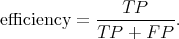
As shown in Fig. 5, galaxies come in a range of different sizes and shapes, or more collectively, morphology. The most well-known system for the morphological classification of galaxies is the Hubble Sequence of elliptical, spiral, barred spiral, and irregular, along with various subclasses [129, 130, 131, 132, 133, 134]. This system correlates to many physical properties known to be important in the formation and evolution of galaxies [135, 136]. Other well-known classification systems are the Yerkes system based on concentration index [137, 138, 139], the de Vaucouleurs [140], exponential [141, 142], and Sérsic index [143, 144] measures of the galaxy light profile, the David Dunlap Observatory (DDO) system [145, 146, 147], and the concentration-asymmetry-clumpiness (CAS) system [148].
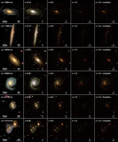 |
Figure 5. Examples of galaxy morphology showing many aspects of the information available to, and issues to be aware of for, a data mining process. These include galaxy shape, structure, texture, inclination, arm pitch, color, resolution, exposure, and, from left to right, redshift, in this case artificially constructed. From Barden, Jahnke & Häußler [151]. |
Because galaxy morphology is a complex phenomenon that correlates to the underlying physics, but is not unique to any one given process, the Hubble sequence has endured, despite it being rather subjective and based on visible-light morphology originally derived from blue-biased photographic plates. The Hubble sequence has been extended in various ways, and for data mining purposes the T system [149, 150] has been extensively used. This system maps the categorical Hubble types E, S0, Sa, Sb, Sc, Sd, and Irr onto the numerical values -5 to 10.
One can, therefore, train a supervised algorithm to assign T types to images for which measured parameters are available. Such parameters can be purely morphological, or include other information such as color. A series of papers by Lahav and collaborators [152, 153, 154, 155, 104, 156] do exactly this, by applying ANNs to predict the T type of galaxies at low redshift, and finding equal accuracy to human experts. ANNs have also been applied to higher redshift data to distinguish between normal and peculiar galaxies [157], and the fundamentally topological and unsupervised SOM ANN has been used to classify galaxies from Hubble Space Telescope images [74], where the initial distribution of classes is not known. Likewise, ANNs have been used to obtain morphological types from galaxy spectra. [158]
Several authors study galaxy morphology at higher redshift by using the Hubble Deep Fields, where the galaxies are generally much more distant, fainter, less evolved, and morphologically peculiar. Three studies [159, 160, 161] use ANNs trained on surface brightness and light profiles to classify galaxies as E/S0, Sabc and Sd/Irr. Another application [162] uses Fourier decomposition on galaxy images followed by ANNs to detect bars and assign T types.
Bazell & Aha [163] uses ensembles of classifiers, including ANN and DT, to reduce the classification error, and Bazell [164] studies the importance of various measured input attributes, finding that no single measured parameter fully reproduces the classifications. Ball et al. [165] obtain similar results to Naim et al. [155], but updated for the SDSS. Ball et al. [166] and Ball, Loveday & Brunner [167] utilize these classifications in studies of the bivariate luminosity function and the morphology-density relation in the SDSS, the first such studies to utilize both a digital sky survey of this size and detailed Hubble types.
Because of the complex nature of galaxy morphology and the plethora of available approaches, a large number of further studies exist: Kelly & McKay [168] (Fig. 6) demonstrate improvement over a simple split in u-r using mixture models, within a schema that incorporates morphology. Serra-Ricart et al. [169] use an encoder ANN to reduce the dimensionality of various datasets and perform several applications, including morphology. Adams & Woolley [170] use a committee of ANNs in a `waterfall' arrangement, in which the output from one ANN formed the input to another which produces more detailed classes, improving their results. Molinari & Smareglia [171] use an SOM to identify E/S0 galaxies in clusters and measure their luminosity function. de Theije & Katgert [172] split E/S0 and spiral galaxies using spectral principal components and study their kinematics in clusters. Genetic algorithms have been employed [173, 174] for attribute selection and to evolve ANNs to classify `bent-double' galaxies in the FIRST [175] radio survey data. Radio morphology combines the compact nucleus of the radio galaxy and extremely long jets. Thus, the bent-double morphology indicates the presence of a galaxy cluster. de la Calleja & Fuentes [176] combine ensembles of ANN and locally weighted regression. Beyond ANN, Spiekermann [177] uses fuzzy algebra and heuristic methods, anticipating the importance of probabilistic studies (Section 4.1) that are just now beginning to emerge. Owens, Griffiths & Ratnatunga [178] use oblique DTs, obtaining similar results to ANN. Zhang, Li & Zhao [179] distinguish early and late types using k-means clustering. SVMs have recently been employed on the COSMOS survey by Huertas-Company et al. [50, 180], enabling early-late separation to KAB = 22 mag twice as good as the CAS system. SVMs will also be used on data from the Gaia satellite [181].
 |
 |
Figure 6. Improvement in classification using a mixture model over that derived from the u and r passbands (u-r color). In this case, the mixture model clearly delineates the third class, which is not seen using u-r. The axes are the first two principle components of the spectro-morphological parameter set (shapelet coefficients in five passbands) describing the galaxies. The light contours are the square root of the probability density from the mixture model fit, and the dark contours are the 95% threshold for each class, in the right-hand panel fitted to the two classes by quadratic discriminant analysis. From Kelly & McKay [168]. |
|
Recently, the popular Galaxy Zoo project [182] has taken an alternative approach to morphological classification, employing crowdsourcing: an application was made available online in which members of the general public were able to view images from the SDSS and assign classifications according to an outlined scheme. The project was very successful, and in a period of six months over 100,000 people provided over 40 million classifications for a sample of 893,212 galaxies, mostly to a limiting depth of r = 17.77 mag. The classifications included categories not previously assigned in astronomical data mining studies, such as edge-on or the handedness of spiral arms, and the project has produced multiple scientific results. The approach represents a complementary one to automated algorithms, because, although humans can see things an algorithm will miss and will be subject to different systematic errors, the runtime is hugely longer: a trained ANN will produce the same 40 million classifications in a few minutes, rather than six months.
3.1.3. Other Galaxy Classifications
Many of the physical properties, and thus classification, of a galaxy are determined by its stellar population. The spectrum of a galaxy is therefore another method for classification [183, 184], and can sometimes produce a clearer link to the underlying physics than the morphology. Spectral classification is important because it is possible for a range of morphological types to have the same spectral type, and vice versa, because spectral types are driven by different underlying physical processes.
Numerous studies [185, 186, 187, 188] have used PCA directly for spectral classification. PCA is also often used as a preprocessing step before the classification of spectral types using an ANN [189]. Folkes, Lahav & Maddox [190] predict morphological types for the 2dF Galaxy Redshift Survey (2dFGRS) [191] using spectra, and Ball et al. [165] directly predict spectral types in the SDSS using an ANN. Slonim et al. [192] use the information bottleneck approach on the 2dFGRS spectra, which maximally preserves the spectral information for the desired number of classes. Lu et al. [193] use ensemble learning for ICA on components of galaxy spectra. Abdalla et al. [194] use ANN and locally weighted regression to directly predict emission line properties from photometry.
Bazell & Miller [82] applied a semi-supervised method suitable for class discovery using ANNs to the ESO-LV [195] and SDSS Early Data Release (EDR) catalogs. They found that a reduction of up to 57% in classification error was possible compared to purely supervised ANNs. The larger of the two catalogs, the SDSS EDR, represents a preliminary dataset about 6% of the final data release of the SDSS, clearly indicating the as-yet untapped potential of this approach. The semi-supervised approach also resembles the hybrid empirical-template approach to photometric redshifts (Section 3.2), as both seek to utilize an existing training set where available even if it does not span the whole parameter space. However, the approach used by Bazell & Miller is more general, because it allows new classes of objects to be added, whereas the hybrid approach can only iterate existing templates.
Most of the emitted electromagnetic radiation in the universe is either from stars, or the accretion disks surrounding supermassive black holes in active galactic nuclei (AGN). The latter phenomenon is particularly dramatic in the case of quasars, where the light from the central region can outshine the rest of the galaxy. Because supermassive black holes are thought to be fairly ubiquitous in large galaxies, and their fueling, and thus their intrinsic brightness, can be influenced by the environment surrounding the host galaxy, quasars and other AGN are important for understanding the formation and evolution of structure in the universe.
The selection of quasars and other AGN from an astronomical survey is a
well-known and important problem, and one well suited to a data mining
approach. It is well-known that different wavebands (X-ray, optical,
radio) will select different AGN, and that no one waveband can select
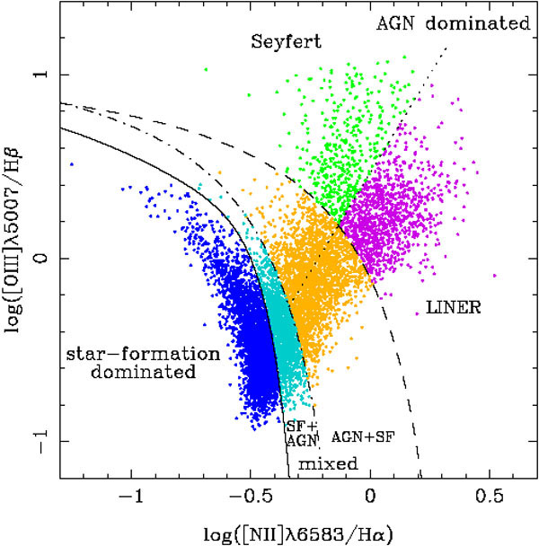
them all. Traditionally, AGN are classified on the
Baldwin-Phillips-Terlevich diagram
[196],
in which sources are plotted on the two-dimensional space of the
emission line ratios
[O III]  5007 /
H
5007 /
H and [N II] /
H
and [N II] /
H , that is separated by
a single curved line into star-forming and AGN regions. Data mining not
only improves on this by allowing a more refined or higher dimensional
separation, but also by including passive objects in the same framework
(Fig. 7). This allows for the probability that
an object contains an AGN to be calculated, and does not require all (or
any) of the emission lines to be detected.
, that is separated by
a single curved line into star-forming and AGN regions. Data mining not
only improves on this by allowing a more refined or higher dimensional
separation, but also by including passive objects in the same framework
(Fig. 7). This allows for the probability that
an object contains an AGN to be calculated, and does not require all (or
any) of the emission lines to be detected.
 |
 |
Figure 7. Upper panel: Baldwin-Philips-Terlevich diagram, which classifies active galactic nuclei (AGN) and star-forming galaxies but requires all four emission lines to be present in the spectrum. From Bamford et al. [212] (although it should be noted that the use of this diagram is not the basis of their study). The axes are the diagnostic emission line ratios from the spectra. Lower panel: AGN/star-forming/passive classification using an ANN, which has no such requirement. The axes are the two outputs from the ANN, e1 and e2 mapped onto (e1,e2) = (e1 + e2/2)i + e2 j, where passive, AGN, star-forming, and hybrid are (0,0), (1,0), (0,1), and (0.5,0.5), respectively. From Abdalla et al. [194]. |
Several groups have used ANNs [197, 198, 199] or DTs [200, 201, 126, 202, 203, 204, 205] to select quasar candidates from surveys. White et al. [200] show that the DT method improves the reliability of the selection to 85% compared to only 60% for simpler criteria. Other algorithms employed include PCA [206], SVM and learning vector quantization [207], kd-tree [208], clustering in the form of principal surfaces and negative entropy clustering [209], and kernel density estimation [210]. Many of these papers combine multiwavelength data, particularly X-ray, optical, and radio.
Similarly, one can select and classify candidates of all types of AGN [211]. If multiwavelength data are available, the characteristic data mining algorithm ability to form a model of the required complexity to extract the information could enable it to use the full information to extract more complete AGN samples. More generally, one can classify both normal and active galaxies in one system, differentiating between star formation and AGN. As one example, DTs have been used [126] to select quasar candidates in the SDSS, providing the probabilities P(star, galaxy, quasar). P(star formation, AGN) could be supplied in a similar framework. Bamford et al. [212] combine mixture modeling and regression to perform non-parametric mixture regression, and is the first study to obtain such components and then study them versus environment. The components are passive, star-forming, and two types of AGN.
Often, the first component of classification is the actual process of object detection, which often is done at some signal-to-noise threshold. Several statistical data mining algorithms have been employed, and software packages written, for this purpose, including the Faint Object Classification and Analysis System (FOCAS) [213], DAOPHOT [214], Source Extractor (SExtractor) [215], maximum likelihood, wavelets, ICA [216], mixture models [217], and ANNs [121]. Serra-Ricart et al. [218] show that ANNs are able to classify faint objects as well as a Bayesian classifier but with considerable computational speedup.
Several studies are more general than star-galaxy separation or galaxy classification, and assign classifications of varying detail to a broad range of astrophysical objects. Goebel et al. [219] apply the AutoClass Bayesian classifier to the IRAS LRS atlas, finding new and scientifically interesting object classes. McGlynn et al. [220] use oblique DTs in a system called ClassX to classify X-ray objects into stars, white dwarfs, X-ray binaries, galaxies, AGN, and clusters of galaxies, concluding that the system has the potential to significantly increase the known populations of some rare object types. Suchkov, Hanisch & Margon [201] use the same system to classify objects in the SDSS. Bazell, Miller & Subbarao [221] apply semi-supervised learning to SDSS spectra, including those classified as `unknown', finding two classes of objects consisting of over 50% unknown.
Stellar classifications are necessarily either spectral or based on color, due to the pointlike nature of the source. This field has a long history and well established results such as the HR diagram and the OBAFGKM spectral sequence. The latter is extended to a two-dimensional system of spectral type and luminosity classes I-V to form the two-dimensional MK classification system of Morgan, Keenan & Kellman [222]. Class I are supergiants, through to class V, dwarfs, or main-sequence stars. The spectral types correspond to the hottest and most massive stars, O, through to the coolest and least massive, M, and each class is subdivided into ten subclasses 0-9. Thus, the MK classification of the sun is G2V.
The use of automated algorithms to assign MK classes is analogous to that for assigning Hubble types to galaxies in several ways: before automated algorithms, stellar spectra were compared by eye to standard examples; the MK system is closely correlated to the underlying physics, but is ultimately based on observable quantities; the system works quite well but has been extended in numerous ways to incorporate objects that do not fit the main classes (e.g., L and T dwarfs, Wolf-Rayet stars, carbon stars, white dwarfs, and so on). Two differences from galaxy classification are the number of input parameters, in this case spectral indices, and the number of classes. In MK classification the numbers are generally higher, of order 50 or more input parameters, compared to of order 10 for galaxies.
Given a large body of work for galaxies that has involved the use of artificial neural networks, and the similarities just outlined, it is not surprising that similar approaches have been employed for stellar classification [223, 224, 225, 226, 227, 228], with a typical accuracy of one spectral type and half a luminosity type. The relatively large number of object attributes and output classes compared to the number of objects in each class does not invalidate the approach, because the efforts described generally find that the number of principal components represented by the inputs is typically much lower. A well-known property of neural networks is that they are robust to a large number of redundant attributes (Section 2.4.5).
Neural networks have been used for other stellar classifications schemes, e.g. Gupta et al. [229] define 17 classes for IRAS sources, including planetary nebulae and HII regions. Other methods have been employed; a recent example is Manteiga et al. [230], who use a fuzzy logic knowledge-based system with a hierarchical tree of decision rules. Beyond the MK and other static classifications, variable stars have been extensively studied for many years, e.g., Wozniak et al. [231] use SVM to distinguish Mira variables.
The detection and characterization of supernovae is important for both understanding the astrophysics of these events, and their use as standard candles in constraining aspects of cosmology such as the dark energy equation of state. Bailey et al. [232] use boosted DTs, random forests, and SVMs to classify supernovae in difference images, finding a ten times reduction in the false-positive rate compared to standard techniques involving parameter thresholds (Fig. 8).
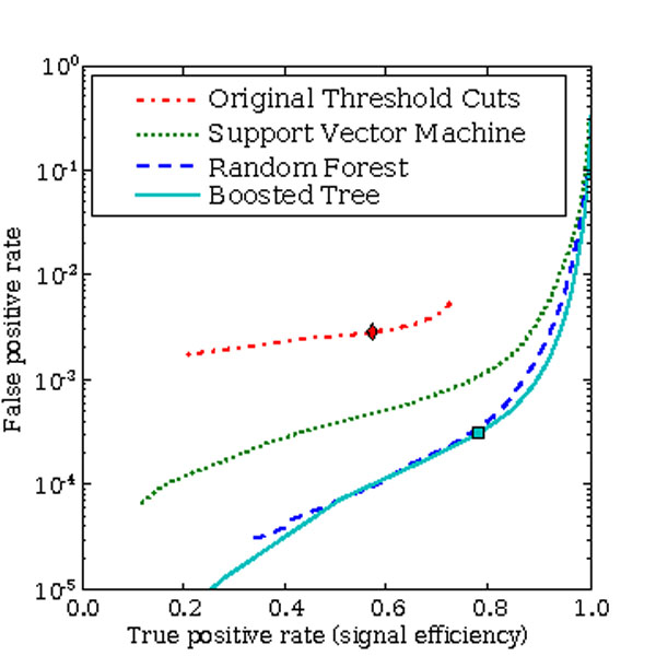 |
Figure 8. Improvement in the classification of supernovae using support vector machine and decision tree, compared to previously used threshold cuts. From Bailey et al. [232]. |
Given the general nature of the data mining approach, there are many further classification examples, including cosmic ray hits [39, 233], planetary nebulae [234], asteroids [235], and gamma ray sources [236, 237].
An area of astrophysics that has greatly increased in popularity in the last few years is the estimation of redshifts from photometric data (photo-zs). This is because, although the distances are less accurate than those obtained with spectra, the sheer number of objects with photometric measurements can often make up for the reduction in individual accuracy by suppressing the statistical noise of an ensemble calculation.
Photo-zs were first demonstrated in the mid 20th century [238, 239], and later in the 1980s [240, 241]. In the 1990s, the advent of the Hubble Space Telescope Deep fields resulted in numerous approaches [242, 243, 244, 245, 246, 247, 248], reviewed by Koo [249]. In the past decade, the advent of wide-field CCD surveys and multifiber spectroscopy have revolutionized the study of photo-zs to the point where they are indispensable for the upcoming next generation surveys, and a large number of studies have been made.
The two common approaches to photo-zs are the template method and the empirical training set method. The template approach has many complicating issues [250], including calibration, zero-points, priors, multiwavelength performance (e.g., poor in the mid-infrared), and difficulty handling missing or incomplete training data. We focus in this review on the empirical approach, as it is an implementation of supervised learning. In the future, it is likely that a hybrid method incorporating both templates and the empirical approach will be used, and that the use of full probability density functions will become increasingly important. For many applications, knowing the error distribution in the redshifts is at least as important as the accuracy of the redshifts themselves, further motivating the calculation of PDFs.
At low redshifts, the calculation of photometric redshifts for normal galaxies is quite straightforward due to the break in the typical galaxy spectrum at 4000A. Thus, as a galaxy is redshifted with increasing distance, the color (measured as a difference in magnitudes) changes relatively smoothly. As a result, both template and empirical photo-z approaches obtain similar results, a root-mean-square deviation of ~ 0.02 in redshift, which is close to the best possible result given the intrinsic spread in the properties [251]. This has been shown with ANNs [33, 165, 156, 252, 253, 254, 124, 255, 256, 257, 179], SVM [258, 259], DT [260], kNN [261], empirical polynomial relations [262, 251, 247, 263, 264, 265], numerous template-based studies, and several other methods. At higher redshifts, obtaining accurate results becomes more difficult because the 4000A break is shifted redward of the optical, galaxies are fainter and thus spectral data are sparser, and galaxies intrinsically evolve over time. The first explorations at higher redshift were the Hubble Deep Fields in the 1990s, described above (Section 3.2), and, more recently, new infrared data have become available, which allow the 4000A break to be seen to higher redshift, which improves the results. Template-based algorithms work well, provided suitable templates into the infrared are available, and supervised algorithms simply incorporate the new data and work in the same manner as previously described.
While supervised learning has been successfully used, beyond the spectral regime the obvious limitation arises that in order to reach the limiting magnitude of the photometric portions of surveys, extrapolation would be required. In this regime, or where only small training sets are available, template-based results can be used, but without spectral information, the templates themselves are being extrapolated. However, the extrapolation of the templates is being done in a more physically motivated manner. It is likely that the more general hybrid approach of using empirical data to iteratively improve the templates, [266, 267, 268, 269, 270, 271] or the semi-supervised method described in Section 2.4.3 will ultimately provide a more elegant solution. Another issue at higher redshift is that the available numbers of objects can become quite small (in the hundreds or fewer), thus reintroducing the curse of dimensionality by a simple lack of objects compared to measured wavebands. The methods of dimension reduction (Section 2.3) can help to mitigate this effect.
Historically, the calculation of photometric redshifts for quasars and other AGN has been even more difficult than for galaxies, because the spectra are dominated by bright but narrow emission lines, which in broad photometric passbands can dominate the color. The color-redshift relation of quasars is thus subject to several effects, including degeneracy, one emission line appearing like another at a different redshift, an emission line disappearing between survey filters, and reddening. In addition, the filter sets of surveys are generally designed for normal galaxies and not quasars. The assignment of these quasar photo-zs is thus a complex problem that is amenable to data mining in a similar manner to the classification of AGN described in Section 3.1.4.
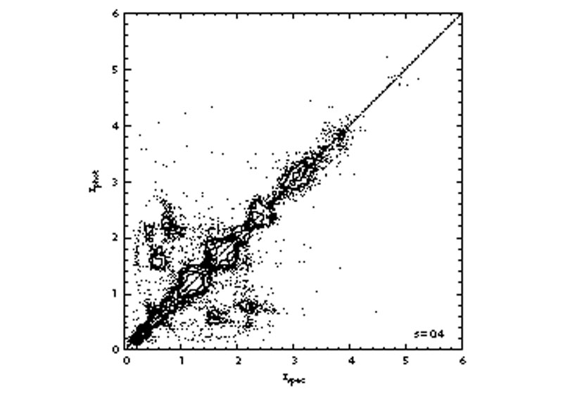
The calculation of quasar photo-zs has had some success using SDSS data [272, 273, 274, 275, 276, 277], but they suffer from catastrophic failures, in which, as shown in Fig. 9, the photometric redshift for a subset of the objects is completely incorrect. However, data mining approaches have resulted in improvements to this situation. Ball et al. [278] find that a single-neighbor kNN gives a similar result to the templates, but multiple neighbors, or other supervised algorithms such as DT or ANN, pull in the regions of catastrophic failure and significantly decrease the spread in the results. Kumar [279] also shows this effect. Ball et al. [261] go further and are able to largely eliminate the catastrophics by selecting the subset of quasars with one peak in their redshift probability density function (Section 4.1), a result confirmed by Wolf [280]. Wolf et al. [281] also show significant improvement using the COMBO-17 survey, which has 17 filters compared to the five of the SDSS, but unfortunately the photometric sample is much smaller.
 |
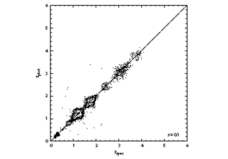 |
Figure 9. Photometric redshift,
zp, vs. spectroscopic redshift, zs,
for quasars in the Sloan Digital Sky Survey, showing, in the upper
panel, catastrophic failures in which zp is very
different from zs. Each individual point represents
one quasar, and the contours indicate areas of high areal point
density. |
Beyond the spectral regime, template-based results are sufficient [282], but again suffer from catastrophics. Given our physical understanding of the nature of quasars, it is in fact reasonable to extrapolate in magnitude when using colors as a training set, because while one is going to fainter magnitudes, one is not extrapolating in color. One could therefore quite reasonably assign empirical photo-zs for a full photometric sample of quasars.
3.3. Other Astrophysical Applications
Typically in data mining, information gathered from spectra has formed the training set to apply a predictive technique to objects with photometry. However, it is clear from this process that the spectrum itself contains a large amount of information, and data mining techniques may be used directly on the spectra to extract information that might otherwise remain hidden. Applications to galaxy spectral classification were described in Section 3.1.3. In stellar work, besides the classification of stars into the MK system based on observable parameters, several studies have directly predicted physical parameters of stellar atmospheres using spectral indices. One example is Ramirez, Fuentes & Gulati [283], who utilize a genetic algorithm to select the appropriate input attributes, and predict the parameters using kNN. The attribute selection reduces run time and improves predictive accuracy. Solorio et al. [284] use kNN to study stellar populations and improve the results by using active learning to populate sparse regions of parameter space, an alternative to dimension reduction.
Although it has much potential for the future (Section 4.2), the time domain is a field in which a lot of work has already been done. Examples include the classification of variable stars described in Section 3.1.5, and, in order of distance, the interaction of the solar wind and the Earth's atmosphere, transient lunar phenomena, detection and classification of asteroids and other solar system objects by composition and orbit, solar system planetary atmospheres, stellar proper motions, extrasolar planets, novae, stellar orbits around the supermassive black hole at the Galactic center, microlensing from massive compact halo objects, supernovae, gamma ray bursts, and quasar variability. A good overview is provided by Becker [285]. The large potential of the time domain for novel discovery lies within the as yet unexplored parameter space defined by depth, sky coverage, and temporal resolution [286]. One constraining characteristic of the most variable sources beyond the solar system is that they are generally point sources. As a result, the timescales of interest are constrained by the light crossing time for the source.
The analysis of the cosmic microwave background (CMB) is amenable to several techniques, including Bayesian modeling, wavelets, and ICA. The latter, in particular via the FastICA algorithm [216], has been used in removal of CMB foregrounds [287], and cluster detection via the Sunyaev-Zeldovich effect [288]. Phillips & Kogut [289] use a committee of ANNs for cosmological parameter estimation in CMB datasets, by training them to identify parameter values in Monte Carlo simulations. This gives unbiased parameter estimation in considerably less processing time than maximum likelihood, but with comparable accuracy.
One can use the fact that objects cross-matched between surveys will likely have correlated distributions in their measured attributes, for example, similar position on the sky, to improve cross-matching results using pattern classifiers. Rohde et al. [290] combine distribution estimates and probabilistic classifiers to produce such an improvement, and supply probabilistic outputs.
Taylor & Diaz [291] obtain empirical fits for Galactic metallicity using ANNs, whose architectures are evolved using genetic algorithms. This method is able to provide equations for metallicity from line ratios, mitigating the `black box' element common to ANNs, and, in addition, is potentially able to identify new metallicity diagnostics.
Bogdanos & Nesseris [292] analyze Type Ia supernovae using genetic algorithms to extract constraints on the dark energy equation of state. This method is non-parametric, which minimizes bias from the necessarily a priori assumptions of parametric models.
Lunar and planetary science, space science, and solar physics also provide many examples of data mining uses. One example is Li et al. [293], who demonstrate improvements in solar flare forecasting resulting from the use of a mixture of experts, in this case SVM and kNN. The analysis of the abundance of minerals or constituents in soil samples [294] using mixture models is another example of direct data mining of spectra.
Finally, data mining can be performed on astronomical simulations, as well as real datasets. Modern simulations can rival or even exceed real datasets in size and complexity, and as such the data mining approach can be appropriate. An example is the incorporation of theory [295] into the Virtual Observatory (Section 4.5). Mining simulation data will present extra challenges compared to observations because in general there are fewer constraints on the type of data presented, e.g., observations are of the same universe, but simulations are not, simulations can probe many astrophysical processes that are not directly observable, such as stellar interiors, and they provide direct physical quantities as well as observational ones. Most of the largest simulations are cosmological, but they span many areas of astrophysics. A prominent cosmological simulation is the Millennium Run [296], and over 200 papers have utilized its data 3.
3 http://www.mpa-garching.mpg.de/millennium Back.
 is the
root-mean-square dispersion between
zp and zs. The use of data mining
techniques, including assigning full probability density functions in
photometric redshift, enables the reduction or elimination of these
catastrophics, as shown in the lower panel. Data based on that from
Ball et al.
[
is the
root-mean-square dispersion between
zp and zs. The use of data mining
techniques, including assigning full probability density functions in
photometric redshift, enables the reduction or elimination of these
catastrophics, as shown in the lower panel. Data based on that from
Ball et al.
[