

Any galaxy survey will observe a particular "window" of the
Universe, consisting of an angular mask of the area observed, and a
radial distribution of galaxies. In order to correct for a spatially
varying galaxy selection function, we translate the observed galaxy
density
 (x)
to a dimensionless over-density
(x)
to a dimensionless over-density
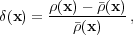 |
(1) |
where  (x) is the expected mean density.
At early times, or on large-scales,
 (x) has a
distribution that is close to that of Gaussian, adiabatic fluctuations
(Planck
Collaboration et al. 2013a),
and thus the statistical distribution is
completely described by the two-point functions of this field.
(x) has a
distribution that is close to that of Gaussian, adiabatic fluctuations
(Planck
Collaboration et al. 2013a),
and thus the statistical distribution is
completely described by the two-point functions of this field.
The correlation function is the expected 2-point function of this statistic
 |
(2) |
From statistical homogeneity and isotropy, we have that
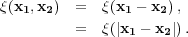 |
(3) |
To help understand the correlation function, suppose that we have two
small regions,
V1 and
V2,
separated by a distance
r. Then the expected number of pairs of galaxies with one galaxy in
V1 and
the other in
V2 is
given by
 |
(4) |
where  is the mean
number of galaxies per unit volume. We see
that
is the mean
number of galaxies per unit volume. We see
that  (r)
measures the excess clustering of galaxies at a
separation r. Imagine throwing down a large number of randomly
placed, equal length r, "sticks" within a survey. Then the
correlation function for that separation r is the excessive fraction
of sticks with a galaxy close to both ends, compared with sticks that
have randomly chosen points within the survey window close to both
ends.
(r)
measures the excess clustering of galaxies at a
separation r. Imagine throwing down a large number of randomly
placed, equal length r, "sticks" within a survey. Then the
correlation function for that separation r is the excessive fraction
of sticks with a galaxy close to both ends, compared with sticks that
have randomly chosen points within the survey window close to both
ends.
If (r)
= 0, the galaxies are unclustered (randomly distributed) on this scale -
the number of pairs is just the expected number of galaxies in
V1
times the expected number in
V2.
Here, the same number of "sticks" have close-galaxies at both ends,
compared with randomly chosen points within the survey window.
(r)
> 0 corresponds to strong clustering, and
(r)
< 0 to anti-clustering. The estimation of
(r)
from a sample of galaxies
will be discussed in Section 4.4.
It is often convenient to measure clustering in Fourier space. In cosmology the following Fourier transform convention is most commonly used
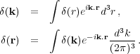 |
(5) (6) |
The power spectrum is defined as
 |
(7) |
with statistical homogeneity and isotropy giving
 |
(8) |
where D is
the Dirac delta function. The correlation
function and power spectrum form a Fourier pair
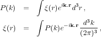 |
(9) (10) |
so they provide the same information. The choice of which to use is therefore somewhat arbitrary (see Hamilton 2005 for a further discussion of this). In order to understand the power spectrum, we need to think about "throwing down" Fourier waves, rather than sticks, but the principle is the same. Methods to calculate the power spectrum from a sample of galaxies are considered in Section 4.3.
The extension of the 2-pt statistics, the power spectrum and the correlation function, to higher orders is straightforward, with Eq. 4 becoming
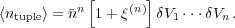 |
(11) |
However, as we will discuss in Section 1.3, at early times and on large scales, we expect the over-density field to have Gaussian statistics. This follows from the central limit theorem, which implies that a density distribution is asymptotically Gaussian in the limit where the density results from the average of many independent processes. The over-density field has zero mean by definition so, in this regime, is completely characterised by either the correlation function or the power spectrum. Consequently, measuring either the correlation function or the power spectrum provides a statistically complete description of the field. Higher order statistics tell us about the break-down of the linear regime, showing how the gravitational build-up of structures occurs and allowing tests of General Relativity.
Although the true Universe is expected to be statistically homogeneous
and isotropic, the observed Universe is not so, because of a number of
observational effects discussed in
Section 5. Statistically, these effect are
symmetric around the line-of-sight and, in the distant-observer limit
possess a reflectional symmetry along the line-of-sight looking
outwards or inwards. Thus, to first order, the anisotropies in the
over-density field can be written as a function of
µ2, where µ
is the cosine of the angle to the line-of-sight. Consequently, we
often write the correlation function
(r,
µ) and the power spectrum P(k, µ).
It is common to expand both the correlation function and power spectrum in Legendre polynomials Lℓ(µ) to give multipole moments,
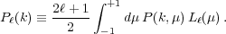 |
(12) |
The first three even Legendre polynomials are L0(µ) = 1, L2(µ) = (3µ2 - 1) / 2 and L4(µ) = (35µ4 - 30µ2 + 3) / 8.