5. OBSERVATIONAL EFFECTS

Up to this point, we have been concerned with comoving galaxy clustering, and the information it contains. In fact, a lot of the information from galaxy surveys does not come directly from the comoving power, but from effects that distort the observed signal away from this ideal. We now outline three of these effects, showing how they can be used to retrieve cosmological information.

5.1. Projection and the Alcock-Paczynski effect

The physics described above is encoded into the comoving galaxy power spectrum. However, we do not measure clustering directly in comoving space, but we instead measure galaxy redshifts and angles and infer distances from these. If we use the wrong cosmological model to do this conversion, then the distances we infer will be wrong and the comoving clustering will contain detectable distortions.

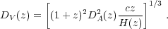
In the radial direction, provided that the clustering signal is small compared with the cosmological distortions, we are sensitive to the Hubble parameter through 1/H(z). In the angular direction the distortions depend on the angular diameter distance D_A(z). Adjusting the cosmological model to ensure that angular and radial clustering match constrains H(z)D_A(z), and was first proposed as a cosmological test (the AP test) by Alcock and Paczynski (1979). If we instead consider averaging clustering in 3D over all directions, then, to first order, matching the scale of clustering measurements to the comoving clustering expected is sensitive to

(33)

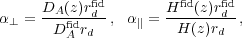
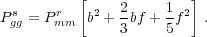
Although this projection applies to all of the clustering signal, BAO provide the most robust and strongest source for the comparison between observed and expected clustering, providing a distinct feature on sufficiently large scales that it is difficult to alter with non-linear physics. In order to extract this information, we need to parametrize over nuisance broad-band features, extracting just the BAO signal. This is usually achieved by means of a smooth function, commonly a polynomial or spline with a set of free parameters, with sufficient flexibility to match the broad-band shape of all of the cosmological models to be tested, but not the BAO signal. If a fiducial cosmological model is used to convert redshifts to distances, then departures between the expected BAO position, and the observed one are commonly quantified by dilation scales. For an anisotropic fit, we can define two dilation scales, perpendicular and parallel to the line-of-sight

(34)

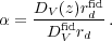
where r_d sets the comoving BAO scale (see Section 2.3), and a superscript fid denotes that a quantity refers to the fiducial cosmology used to measure the clustering signal. For a single fit to the BAO in an isotropically averaged clustering measurement, the combined dilation scale is

(35)

Estimates of the BAO scale can be made based on either (r) or P(k), but they include the noise from small scales and shot noise differently. Anderson et al. (2012) averaged measurements made from both statistics, using mocks to show that this improved the combined error.

A review of current BAO measurements was provided in the introduction of Anderson et al. (2012), which described recent experiments (e.g. Beutler et al. 2011, Blake et al. 2011, Padmanabhan et al. 2012), leading to the analyses presented in Anderson et al. (2012). Since then, the DR9 data set has been analysed splitting into measurements along and across the line-of-sight (Anderson et al. 2013), and the next release of measurements from BOSS is imminent. In addition, the range of redshifts covered by BAO measurements has increased further, through BOSS analyses using the Lyman-α forest in quasar spectra (Busca et al. 2013, Slosar et al. 2013, Kirkby et al. 2013).

5.2. Redshift-space distortions

The second observational effect that we will consider results from the fact that our estimates of galaxy distances are made from redshifts. These redshifts are caused by both the Hubble expansion and from any additional motion within a comoving frame, called the peculiar velocity. We can write

(36)

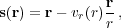
where s is the redshift-space (i.e. derived from the redshift) position of a galaxy, r is the true real-space position of the galaxy away with the observer at the origin, and v_r(r) is the radial component of the peculiar velocity. The distortions in the field that result from the peculiar-velocity dependent shifts are called Redshift-Space Distortions (RSD).

Locally, galaxies act as test particles in the flow of matter. If galaxies fully sampled the velocity field, the peculiar velocity distribution of galaxies would match that of the mass. We should be aware that galaxies are expected to be at special locations in the density field, potentially giving rise to a small bias in their velocity distribution compared to that of the mass.

As discussed in Section 3.1, structures are continually growing through gravity. On large-scales this growth is the dominant source of RSD. Consider a galaxy on the near-edge of a strong over-density: this galaxy will tend to be falling in to the over-density, away from us, increasing its redshift and moving its apparent position closer to the centre of the over-density. A galaxy at the far-edge of an over-density will appear closer, and we therefore see that clusters will appear "squashed" along the line-of-sight in redshift-space. By a similar argument, under-dense regions appear "stretched" along the line-of-sight. This is shown in Fig. 6.

Figure 6. Explanatory diagram showing how real-space structures (top row) look in redshift-space (bottom row).

If we assume that the patch of the Universe from which clustering is measured is sufficiently far away that the line-of-sight is approximately constant across the patch, this effect causes an increase in the measured power that can be easily modelled. Following Kaiser (1987), on linear scales we can derive a change in the power corresponding to

(37)

where = ∇ ⋅ v is the divergence of the peculiar velocity field, a superscript s denotes that a quantity is measured in redshift-space and r in real-space, and a subscript g denotes that a quantity refers to the galaxy field. Furthermore, in the linear regime, we can write = -f_m, where m refers to the matter field, and

(38)

is the logarithmic derivative of the linear growth rate. Assuming a linear bias, we can write _g^r = b _m^r, and we see that the amplitude of the anisotropic power spectrum given in Eq. (37) depends on b₈ and f₈, where ₈ is the standard deviation of the distribution of over-densities when averaged over spheres of radius 8 Mpc h^-1. If we spherically average the power spectrum, equivalent to integrating over 0 < µ < 1, we find that

(39)

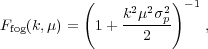
On small-scales, there is a second RSD effect caused by galaxy motion within collapsed objects with deep potential wells. The random velocities attained by such galaxies smear the collapsed object along the line of sight in redshift space, leading to the existence of linear structures pointing towards the observer in redshift-space. This is shown in Fig. 6. These apparent structures are known as "Fingers-of-God" (FoG) and reduce information on small scales. If the pairwise velocity dispersion within a collapsed object has an exponential distribution (superposition of Gaussians), then we get a multiplicative damping term for the power spectrum of the form

(40)

where _p ~ 400 km s^-1 (Hawkins et al. 2003). It is common to multiply P_gg^s(k, µ) from Eq. (37) by F_fog(k, µ) to provide a combined model for the anisotropic power spectrum. However this model is not guaranteed to work in the quasi-linear regime, although the damping term can model some of the quasi-linear signal if _p is treated as a free parameter (Percival and White 2009).

An alternative to modelling the FoG is to try to correct data by using phase information to "collapse clusters" along the line of sight (e.g. Tegmark et al. 2004). This method has similarities with "reconstruction" used to recover BAO information. For the SDSS-II Luminous Red Galaxy sample, Reid et al. (2010) used an anisotropic friends-of-friends group finder, normalised using numerical simulations (Reid et al. 2009) to locate clusters and move the galaxies to the average redshift, removing much of the FoG signal and reducing the modelling burden.

Standard measurements of the RSD signal are intrinsically limited by the number of radial modes present, which provide the sample variance limit. McDonald and Seljak (2009) showed that, with two samples of galaxies covering the same region, it is possible to measure ratios of power spectra independent of cosmic variance - provided that the two samples both have different linear deterministic biases. Taking into account the anisotropic nature of their redshift-space power spectrum, shot-noise limited measurements of f / b_i and b_i / b_j (where i,j refer to the galaxy samples) would be possible. These combine to give measurements of f₈ that are limited by the total number of modes within a survey, rather than just those in the radial direction - potentially a strong source of further information.

The picture for RSD measurements presented in this section relies on a number of assumptions, particularly the combination of linear theory with a simple damping model, and the assumption that we are only interested in pairs of galaxies for which the line-of-sights are approximately parallel. These assumptions have been tested and shown to be adequate for current RSD growth rate measurements (Samushia et al. 2012). Many RSD-based measurements of the growth rate have been made from a number of spectroscopic surveys, with a recent compilation provided in Reid et al. (2012).

5.3. Joint AP and RSD measurements

The primary problem with making RSD and AP measurements of the full (not just BAO) clustering signal is disentangling both effects (Ballinger et al. 1996), although Samushia et al. (2012) showed how future surveys ameliorate this problem. For current surveys, this separation can only be achieved on large-scales, where RSD can be modelled with perturbation theory, leading to joint RSD and AP measurements (e.g. Reid et al. 2012). The power of the large-scale AP test was shown in Samushia et al. (2013), who demonstrated that using the joint H(z) and D_A(z) AP measurements of Reid et al. (2012) led to a fortuitous degeneracy breaking compared with using the isotropic BAO measurements of Anderson et al. (2012). This led to a factor of five improvement on measuring the Dark Energy equation-of-state w(z = 0.57), which is particularly impressive given that the same data were used to make both measurements.

5.4. Primordial non-Gaussianity

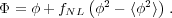
As discussed in Section 2, determining the amount of primordial non-Gaussianity in the matter over-density field provides a key way of distinguishing between inflationary models. Observations of the large-scale clustering of galaxies have the potential to measure this, as we will now demonstrate. One of the simplest way to parameterise non-Gaussianity is to assume that the potential has a local quadratic term

(41)

Although many other forms of non-Gaussianity are possible, any detection of non-Gaussianity would be interesting, and it is therefore instructive to consider how this simple model can be constrained by galaxy clustering measurements (Dalal et al. 2008).

We can see this by reconsidering the peak-background split model - in Section 3.4, we saw that halo formation is much easier with additional long-wavelength fluctuations. If we decompose the potential in Eq. (41) into long (_l) and short (_s) wavelength components, we find that

(42)

The f_NLl² term is small, but we see that there is an extra term 2f_NLls, which is of importance for the large-scale bias. To see how this enters into the peak-background split model, note that the link between over-density and potential can be written _l(k) = α(k)(k), where

(43)

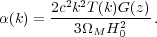
Now, one factor of α gets absorbed into converting one of the potentials in the extra term to an over-density, but we are left with a critical density that is modulated not just by the Gaussian long-wavelength fluctuation, but by

(44)

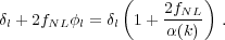
This extra term propagates into the change in number density of haloes and the bias as determined by the peak-background split model

(45) (46)

Because of the k² term in α(k), the bias diverges to large-scales, giving a detectable signature with amplitude dependent on f_NL.

Unfortunately, the large-scale clustering signal is one of the most difficult to measure, not just because large volumes are required to reduce sample variance. In fact, observational systematics can strongly affect the clustering on large-scales. For the SDSS, variations in stellar density and seeing for imaging data can lead to target density fluctuations giving rise to large-scale power in spectroscopic galaxy samples that is degenerate with the f_NL signature (Ross et al. 2011, Ross et al. 2012). Current galaxy survey measurements of local f_NL are consistent with f_NL = 0, with contraints from galaxy surveys giving measurements of f_NL ± 21 at 1 (Giannantonio et al. 2013), which should be compared with those from the CMB, which are of order ± 5 (Planck Collaboration et al. 2013a).

5.5. Summary

A summary of the physics encoded within the linear galaxy power spectrum is presented in Fig. 7. This provides a simple model for the power spectrum, showing the measurements that can be made from each component.

Figure 7. Summary of the physics encoded in the observed large-scale galaxy clustering signal, as described by the linear power spectrum.