


Supernovae (which we will often abbreviate to SN or SNe) are the most straightforward tool for studying cosmic acceleration, and they are the tool that directly discovered acceleration in the first place (Riess et al. 1998, Perlmutter et al. 1999; both using local calibration samples from the Cal`n/Tololo survey, Hamuy et al. 1996). Type Ia supernovae, defined observationally by the absence of hydrogen and presence of SiII in their early-time spectra (Filippenko 1997), are thought to arise from thermonuclear explosions of white dwarfs, though the evolutionary sequence or sequences that lead to these explosions remains poorly understood. The two broad classes of progenitor models are "single degenerate," in which a white dwarf accreting from a binary companion is pushed over the Chandrasekhar mass limit, and "double degenerate," in which gravitational radiation causes an orbiting pair of white dwarfs to merge and exceed the Chandrasekhar mass. The observed supernova population could have contributions from both channels (see Livio 1999 for a review of Type Ia SN mechanisms).
To a rough approximation, Type Ia SNe are standard candles, with rms dispersion of approximately 0.4 magnitudes in V-band at peak luminosity (Hamuy et al. 1996, Riess et al. 1996). This 0.4-mag scatter can be sharply reduced using an empirical correlation between peak luminosity and light curve shape (LCS) — supernovae with higher peak luminosities decline more slowly after the peak. This correlation, which we will refer to generically as the luminosity-LCS relation, was first quantified by Phillips (1993) based on a handful of objects including the archetypes of low and high luminosity Ia supernovae, SN 1991bg and SN 1991T, respectively. Also important to the refinement of distance determinations was the development of corrections for the correlation between SN color and extinction (Riess et al. 1996, Tripp 1998, Phillips et al. 1999) and K-corrections for redshifting effects (Kim et al. 1996, Nugent et al. 2002). These were all quickly incorporated into analysis methods such as the Multicolor Light Curve Shape (MLCS; Riess et al. 1996) technique used by the High-z Supernova Search (Schmidt et al. 1998) and the stretch-factor formalism used by the Supernova Cosmology Project (Perlmutter et al. 1997).
With these corrections, the dispersion in well measured optical band peak magnitudes is only ~ 0.12 magnitudes (Hicken et al. 2009b, Folatelli et al. 2010), allowing each well measured supernova to provide a luminosity-distance estimate with ~ 6% uncertainty. The diversity of SN Ia light curves is not fully understood, and peculiar SNe Ia appear to produce ~ 5% non-Gaussian tails in the SN Ia distribution (Li et al. 2011). For the bulk of the population, the prevailing picture is that the progenitor explosions produce varying amounts of Ni56, whose radioactivity powers the optical luminosity, and that the correlation of peak luminosity with light curve shape arises from radiative transfer effects (Hoeflich et al. 1996, Kasen and Woosley 2007). Recent studies suggest that SN Ia are truly standard candles in the near-IR, with peak luminosities at rest-frame H-band (1.6 μm) that have only ~ 0.1 magnitude rms dispersion independent of light curve shape, and with little sensitivity to uncertain reddening laws (Mandel et al. 2009, Mandel et al. 2011, Barone-Nugent et al. 2012). This small dispersion in near-IR peak luminosities relative to optical is consistent with theoretical expectations from radiative transfer models (Kasen 2006).
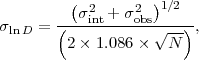
To measure cosmic expansion with Type Ia SNe, one compares the corrected peak apparent magnitudes of distant supernovae to those of local calibrators at 0.03 < z < 0.1, a "sweet spot" in which distances inferred from redshifts are insensitive to peculiar velocities and to the assumed densities of dark matter and dark energy. Since the distances to the local calibrators are usually determined from Hubble expansion, this method gives the luminosity distance DL in units of h-1 Mpc. More generally, the SN method yields relative distances in different redshift bins, even if one of those bins is not strictly local. The DL(z) relation is sensitive to dark energy through equations (7) and (3), and to space curvature through equations (10) and (11). A measurement of N supernovae in a redshift bin with rms observational errors σobs in peak magnitudes yields an estimate of DL(z) with fractional statistical error
 |
(51) |
where σint is the rms intrinsic scatter, the factor 1.086 converts from magnitudes to natural logarithms, and the factor of two converts from flux uncertainty to distance uncertainty. As discussed in Section 3.4 below, there are many possible sources of systematic uncertainty, including flux calibration, corrections for dust extinction, and possible redshift evolution of the supernova population. Of these, dust extinction looks like it may ultimately be the most difficult to control at the sub-percent level, since even a 0.01-mag E(B - V) color excess corresponds to a 3% suppression of V-band flux. This consideration provides strong motivation for focusing Stage IV supernova surveys on rest-frame near-IR photometry, where dust extinction is a factor of 3 to 8 times smaller compared to the optical and where the small scatter in peak luminosities may help minimize any evolutionary effects.
3.2. The Current State of Play
Building on the initial discovery of cosmic acceleration, supernova surveys have been a major area of activity in observational cosmology over the last decade. The largest high-redshift (z ≈ 0.4-1.0) data sets are those from the ESSENCE survey (Wood-Vasey et al. 2007; Narayan et al., in prep.; ~ 200 spectroscopically confirmed Type Ia SNe) and the CFHT Supernova Legacy Survey (SNLS; Astier et al. 2006, Conley et al. 2011, Sullivan et al. 2011; ~ 500 spectroscopically confirmed Type Ia SNe in the three-year data set SNLS3). At very high redshifts, HST surveys (Riess et al. 2004, Riess et al. 2007, Suzuki et al. 2012) have yielded ~ 25 Type Ia SNe at z > 1.0, which confirm the expectation that the universe was decelerating at high redshift and limit possible systematic effects from evolution of the supernova population or intergalactic dust extinction. At intermediate redshifts (0.1 < z < 0.4), the SDSS-II supernova survey (Frieman et al. 2008, Sako et al. 2008) has discovered and monitored 500 spectroscopically confirmed Type Ia SNe; only the first-year data set (103 SNe) has so far been subjected to a full cosmological analysis (Kessler et al. 2009), but Campbell et al. (2012) present cosmological results from a sample of 752 photometrically classified SDSS-II SNe with spectroscopic host galaxy redshifts, and a joint analysis of the SNLS and SDSS-II samples is in process (J. Frieman, private communication). Finally, the last five years have also seen major efforts to expand the sample of local calibrators and improve their measurements, including rest-frame IR and rest-frame UV photometry (Wood-Vasey et al. 2008, Stritzinger et al. 2011, Contreras et al. 2010, Hicken et al. 2009a).
The greatest cosmological utility from SNe Ia generally comes from the joint use of numerous samples that span a wide range in redshift. To limit systematic errors introduced by combining disparate SN surveys, it is often valuable to recompile a sample from these surveys as homogeneously as possible. This involves applying consistent criteria for inclusion in the sample, light curve fitting with a single algorithm, propagation of errors via covariance matrices, consistent use of K-corrections, and so forth. While any such "survey of surveys" is not unique and may not be optimal for a specific application, these compilations are popular because of their ease of use. Recent examples include the "Gold" sample (Riess et al. 2004, 2007), the "Union" and "Union2" samples (Kowalski et al. 2008, Amanullah et al. 2010), the "Constitution" sample (Hicken et al. 2009a), and the compilation of local, SDSS-II, SNLS3, and HST supernovae analyzed by Conley et al. (2011).
Figure 5 plots luminosity distance measurements from the Union2 compilation over the model predictions shown previously in Figure 2 (multiplied by 1 + z to convert comoving angular diameter distance to luminosity distance). The data are in good agreement with the fiducial cosmological model, and the parameter changes in the bottom panel (Ωk = ± 0.01, 1 + w = ± 0.1) are at the border of detectability. (Recall that other parameters are adjusted to reproduce the CMB anisotropy of the fiducial model; see Table 1.)
 |
Figure 5. Luminosity distance vs. redshift for our fiducial cosmological model (solid curves), superposed on supernova measurements from the Union2 compilation (Amanullah et al. 2010). The lower panel shows residuals from the fiducial model prediction for the SN data, with open circles marking medians of the data in Δz = 0.2 bins and broken curves showing the CMB-normalized variant models described in Table 1. Note that these distances are in h-1 Gpc units. |
Figure 6 illustrates model constraints from the Union2 supernova data and WMAP7 CMB data, which we have computed using CosmoMC (Lewis and Bridle 2002). We use the Union2 covariance matrix that includes correlated systematic error contributions. Panel (a) shows the (Ωm, ΩΛ) plane assuming w = -1. CMB and SN constraints are highly complementary in this plane because the former are most sensitive to the total energy density (Ωm + ΩΛ) and the latter to the difference between the densities of "attractive" matter and "repulsive" dark energy. Together the two data sets yield tight constraints in this space, Ωm = 0.282 ± 0.037, ΩΛ = 0.723 ± 0.030, consistent with a flat universe. Panel (b) shows the (Ωm, w) plane, where we now assume spatial flatness and a constant value of w. Here again the SN and CMB data are highly complementary, yielding a tight combined constraint Ωm = 0.270 ± 0.023, w = - 1.007 ± 0.081, consistent with a cosmological constant. Panel (c) shows the (w0.5, wa) plane, where we have adopted the 2-parameter dark energy model of equation (24); w0.5 is the value of w at z = 0.5, which is much better determined than the value of w0 and only weakly correlated with wa. Here we have assumed spatial flatness and marginalized over uncertainty in Ωm. CMB and SN data provide only weak constraints individually in this model space, but the combination still provides a good constraint on w0.5, with the error on w0.5 = -1.008 ± 0.132 only degraded by ~ 50% compared to panel (b). Constraints on wa, on the other hand, are very weak. The w and w0.5 constraints in panels (b) and (c) would degrade substantially if we allowed non-zero Ωk; with this level of flexibility, one must bring in additional data to get useful constraints. However, an H0 or BAO constraint at the level of current measurements is sufficient to remove most of the sensitivity to Ωk (Mortonson et al. 2010).
 |
Figure 6. Constraints from WMAP7 CMB data, Union2 SN data, and the combination of the two, in (a) the (Ωm, ΩΛ) plane assuming w = -1, (b) the (Ωm,w) plane assuming Ωk = 0, and (c) the (w0.5,wa) plane assuming Ωk = 0, where w0.5 is the value of w at z = 0.5. Contours show 68% confidence intervals. In contrast to panels (a) and (b), the combined contour in (c) is tighter than one would guess from the overlap of the individual contours because the combined data set breaks degeneracies among other parameters that are marginalized over when inferring w0.5 and wa. |
Plots and constraints similar to Figures 5 and 6 appear in many of the papers cited above. The most up-to-date analysis is that of Conley et al. (2011), who find w = -0.91-0.20+0.16(stat)-0.14+0.07(sys) for SNe alone, assuming a flat universe with constant w and marginalizing over Ωm. Combining this measurement with other data sets, Sullivan et al. (2011) find w = -1.016-0.079+0.077 in combination with 7-year WMAP CMB constraints (similar to the value and error bar quoted above), and w= -1.061-0.068+0.069 after adding BAO and H0 measurements.
There are several indications that current SN cosmology studies are limited by systematic uncertainties associated with the linked issues of dust extinction, SN colors, and photometric calibration. In any cosmological analysis, one uses the color of a supernova relative to a template expectation (derived from a training set) to infer, and correct for, a correlation between color and apparent magnitude arising from dust and/or intrinsic color variations. In the analysis of Wood-Vasey et al. (2007), different priors about host galaxy extinction change the inferred value of w by amounts comparable to the statistical error. When the ratio of extinction to reddening is treated as a free parameter in the cosmological fits, the derived values are typically quite far from those measured for Galactic interstellar dust, e.g., RV ≡ AV / E(B - V) = 1.5-2.5 (Hicken et al. 2009b, Kessler et al. 2009, Sullivan et al. 2011) instead of the mean RV = 3.1 found in the diffuse interstellar medium of the Milky Way (Cardelli et al. 1989). This difference could be a reflection of different kinds of dust along the line of sight to the supernova (e.g., circumstellar dust), but it could also arise from intrinsic color differences among SNe Ia with similar light curve shapes, which would reduce the inferred RV if they are assumed to arise from reddening. Supporting the latter idea, the distribution of SN colors shows little dependence on host galaxy properties (Kessler et al. 2009, Sullivan et al. 2010), while such dependence might be expected if the color distribution is strongly affected by dust. Chotard et al. (2011), using spectroscopic indicators of luminosity in nearby SNe, infer an extinction law with RV = 2.8 ± 0.3, consistent with the Galactic value.
One of the main surprises in the first-year analysis of the SDSS-II Supernova Survey (Kessler et al. 2009) was the realization that the two main algorithms developed by other groups for global fitting of SN light curves and cosmological parameters — MLCS2k2 (Jha et al. 2007) and SALT2 (Guy et al. 2007) — initially gave statistically inconsistent cosmological results (w = -0.76 ± 0.07 vs. w = -0.96 ± 0.06, quoting only the statistical errors) when applied to the same data sets, a discrepancy that persisted even if the SDSS-II data themselves were omitted from the fits. Kessler et al. (2009) traced this discrepancy to two factors, one related to calibration data and the other to the treatment of SN colors. For the calibration data, ultraviolet flux measurements in the local sample from the U-band appear inconsistent with those from the g-band at only moderate redshift and suggest a problem with the (observed frame) U-band calibration. 22 This problem translates into a difference between fitters because one is trained with U-band data and the other is not. A more subtle difference arises from the determination of the correction to SN brightness from color measurements, specifically whether the correlation can be assumed to be independent of redshift and survey and whether changes in color are due solely to extinction. While these systematic uncertainties will certainly be reduced by larger multi-wavelength data sets and improved analysis methods, the experience from these recent studies argues strongly for using rest-frame IR photometry in precision cosmological studies to circumvent uncertainties related to extinction.
3.3. Observational Considerations
There are several steps to a supernova cosmology campaign: discovery, monitoring, spectroscopic confirmation, and calibration against low redshift samples. In large area surveys, discovery and monitoring are usually done together, through repeated imaging of a large field of view in multiple bands. A variety of image-differencing techniques can be used to identify SNe (distinguished from other variable objects by their light curves) and measure their magnitudes vs. time. As a rule of thumb, a minimum rest-frame cadence of one observation per ~ 5 days 23 is needed to get adequate measurements of light curve shapes and normalizations, such that statistical errors are dominated by the intrinsic dispersion of SN luminosities and not by observational errors. The required cadence may be somewhat lower in the rest-frame IR, where the dependence on light curve shape is weaker, but one must still have enough data points to determine peak luminosity accurately. At least two bands are needed to measure SN colors and thereby infer dust extinction, though more are better, and multiple colors may prove critical to distinguishing different forms of extinction (interstellar, circumstellar, and intergalactic) from each other and from intrinsic color differences.
Figure 7, based on Table 7 of Tonry et al. (2003), plots the peak apparent magnitude of a typical Type Ia supernova vs. redshift in observed frame I and J band. As a rough rule of thumb, a survey with periodic and uniform exposures targeting supernovae at a given redshift should measure to a signal-to-noise ratio of ~ 15 at peak, so that it still usefully measures the SN before or after peak when it is 1.5 magnitudes fainter. This depth ensures that incompleteness for supernovae below the median luminosity does not bias the results and that photometric errors do not dominate over intrinsic scatter in cosmological analysis. Ground-based surveys designed to observe SNe Ia to z < 0.8 will typically find ~ 10 SNe Ia per square degree per month.
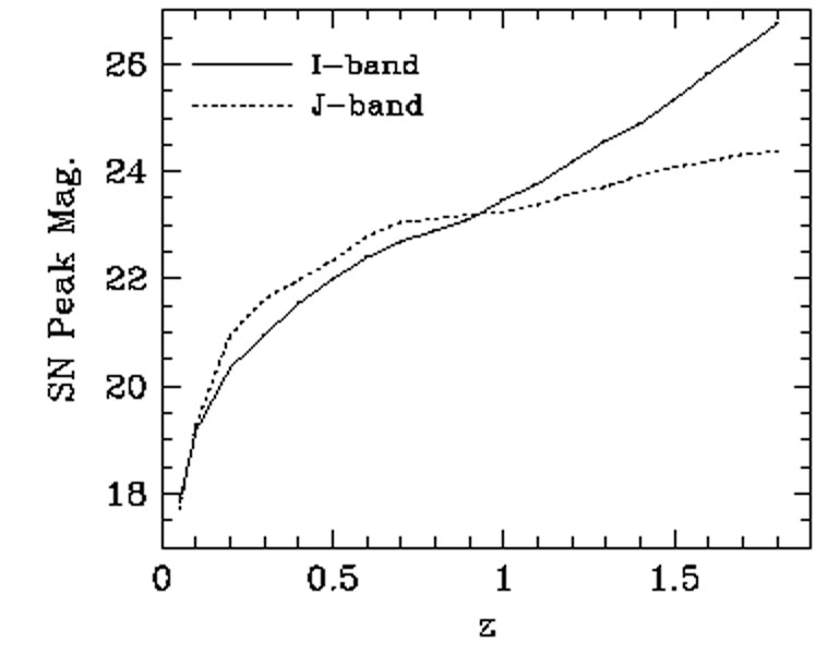 |
Figure 7. Peak apparent magnitude of a typical Type Ia supernova as a function of redshift in observed-frame I-band (solid) or J-band (dotted), from Table 7 of Tonry et al. (2003). The z > 1.1 portion of the I-band curve and z < 0.4 portion of the J-band curve rely on extrapolation of the template systems' spectral energy distributions beyond the observed range. Magnitudes are on the Vega system. |
After discovering SNe, one must determine their type and redshift. The most reliable approach is to obtain their spectra to cross-correlate their spectral features with known templates. Spectral resolution R ~ 250 and S/N ~ 5 per resolution element are adequate for these purposes, but even at this level spectroscopic follow-up is typically the most resource intensive step of a supernova campaign. For the same telescope aperture, an epoch of spectroscopy requires an order of magnitude more time than an epoch of photometry, and one generally loses the parallelism afforded by photometric monitoring with a large camera (which has several SNe per field of view at a given time). Spectroscopic follow-up of the SNLS3 sample, for example, used more than 1600 hours of 8-10m telescope time (M. Sullivan, private communication).
In principle, photometric redshifts can be used in place of spectroscopic redshifts, and if they are accurate to a fractional distance error ΔD / D < 10% they lead to only moderate degradation in statistical accuracy. However, given the degeneracies among redshift, SN color, and dust extinction, and the increased ambition of SN surveys to control systematics, we are skeptical that cosmological SN surveys can achieve the desired accuracy using only broad-band photometric monitoring and spectroscopic follow-up of a small fraction of the sample. An intermediate approach that may work would be to measure the cross-correlation of a supernova SED with the SN Ia spectral features using custom-designed optical filters that are matched to SN spectroscopic features at different redshifts (Scolnic et al. 2009). It also may be possible to make use of subsamples of SNe found in passive (non-star-forming) galaxies, which should host only Type Ia SNe and which allow more accurate photometric redshifts from host galaxies. For type identification, one can also check for a second peak in the rest frame infrared light curve, a morphological feature that is unique to SNe Ia.
Another intermediate approach is to obtain eventual spectroscopic observations of all host galaxies in the cosmological analysis sample but not attempt real-time spectroscopy of all candidate Type Ia supernovae. This scheme still yields precise redshifts, and it provides host galaxy data that can be used to measure and remove correlations between supernova and host galaxy properties (see Section 3.4). While it still requires one faint-object spectrum per supernova, the scheduling demands are much more flexible. One can also apply data quality and other selection cuts before the spectroscopic observations to reduce the total number of spectra required, though one must be careful not to let biases creep in at this stage. With good photometric monitoring and with subsequent spectroscopic redshifts of apparent hosts, Kessler et al. (2010) find that they can identify Type Ia SNe with 70% to 90% confidence from the LCS and color alone, and Bernstein et al. (2012) forecast Type Ia purity as high as 98% for DES-like photometric observations. A moderate amount of real-time supernova spectroscopy may then suffice to assess efficiency and biases. The recent SDSS-II analysis by Campbell et al. (2012) puts this approach into practice, illustrating its promise and its challenges.
Given the photometric and spectroscopic measurements for a selected set of supernovae, one must fit the data set to infer cosmological parameters. Many of the algorithms in current use are descendants of the Multicolor Light Curve Shape (MLCS; Riess et al. 1996) or Spectral Adaptive Light Curve Template (SALT; Guy et al. 2005) methods. In current implementations, MLCS fitters are "trained" on local supernovae to determine the relationships between multi-band light curve shapes and peak absolute magnitudes, and these relationships are applied to distant supernovae to measure DL(z). SALT-style fitters (which include the SiFTO (Conley et al. 2008) algorithm applied to SNLS3) instead apply a global, simultaneous fit of parameters describing cosmology and the relationship between supernova light curves and absolute magnitude. Of greater practical import, however, is the different treatment of supernova colors in the two methods. MLCS fitters attribute color differences at fixed peak luminosity to dust reddening, and they adopt an explicit prior for the distribution of reddening values. SALT fitters allow scatter in intrinsic colors at fixed peak luminosity and do not attempt to separate intrinsic variations from dust reddening. In reality, there certainly are intrinsic color variations at some level, but there is also useful information in the fact that dust reddening exists and has specific properties, in particular that it cannot be negative. An optimal approach should therefore allow for both effects. Bayesian fitting methods (e.g., Mandel et al. 2009, Mandel et al. 2011, March et al. 2011) can in principle incorporate a wide variety of parameterized relationships with explicit priors, including dependences on redshift or host galaxy parameters, which are then marginalized over in cosmological fits. At the level of precision of current SN samples, the differences in fitting methods do matter (e.g., Kessler et al. 2009), so this remains an area of active research. Fortunately, the growing samples of well observed local and distant SNe provide increasingly powerful data to guide this development.
The detailed spectra of SNe could potentially improve their luminosity and/or color calibration relative to photometric light curves alone. For example Foley et al. (2011) find a correlation between intrinsic color and the ejecta velocity inferred from the line width (see also Blondin et al. 2012, Foley 2012). However, Silverman et al. (2012), considering a variety of spectral indicators, find only marginal evidence for a diagnostic that improves Hubble residuals, and Walker et al. (2011) find similarly ambiguous results. Given the substantial observing time required to measure good spectroscopic diagnostics for high redshift SNe, modest reductions in scatter are unlikely to win over simply observing more supernovae. However, spectral diagnostics merit continued investigation to see whether matching spectral properties between high and low redshift SNe can reduce susceptibility to evolutionary systematics.
3.4. Systematic Uncertainties and Strategies for Amelioration
The largest current supernova surveys have ~ 500 Type Ia supernovae. Future surveys hope to discover and monitor thousands of supernovae, sufficient to yield statistical errors of 0.01 mag or smaller in narrow redshift bins with Δz ~ 0.1-0.2. Realizing the statistical power of such surveys will require eliminating or limiting several distinct sources of systematic error. These include flux calibration errors across a wide range of flux and redshift, the systematics associated with SN colors and dust extinction, the possible evolution of the supernova population with redshift, and gravitational lensing. We discuss each of these issues in turn. 24
The leverage of SN studies comes from comparing SNe over a wide span of redshift and thus an enormous range of flux; for example, the typical peak I-band magnitude at z = 0.8 is 23 mag while the median peak B-band magnitude of the local calibrator sample used in many analyses is 17 mag, implying a ratio of 250 in flux. Maintaining sub-percent accuracy in relative flux calibration over such a range would be challenging under any circumstances, and for SN surveys it is complicated by the fact that (a) local and distant SNe are usually observed with different telescopes equipped with different filters, (b) a given observed-frame filter intercepts a different portion of the SN rest-frame spectral energy distribution (SED) at each redshift, and (c) supernova SEDs are very different from those of the standard stars used for flux calibration in most of astronomy. Conley et al. (2011) identify calibration as the dominant systematic in SNLS3, the only systematic in their analysis that makes a major contribution to their total error budget. Flux calibration uncertainties can be reduced by carefully designing photometric SN surveys with specialized hardware (e.g., tunable lasers, NIST photodiodes and calibration sources; Stubbs and Tonry 2006) to measure the system throughput in situ and by choosing filter systems that provide a good match in rest-frame SED sampling between low- and high-redshift samples. The ACCESS rocket program should improve flux calibration with sub-orbital flights that compare NIST photodiodes to calibration stars (Kaiser et al. 2010). "Self-calibration" that marginalizes over flux-calibration uncertainty can further reduce this systematic error (Kim and Miquel 2006), but at the price of increasing statistical error.
As already noted in Section 3.2, uncertainties in dust extinction, linked to uncertainties in intrinsic SN colors and in photometric calibration, are already important systematics in SN studies of cosmic acceleration. These uncertainties can likely be reduced with detailed, well calibrated, multi-wavelength observations of large numbers of low redshift SNe, which can characterize the separate dependence of SN colors on luminosity, light curve shape, and time since explosion, and provide constraints on dust extinction laws that are isolated from cosmological inferences. The final analyses of data from the SDSS-II supernova survey (Frieman et al. 2008) and the low-redshift portion of the Carnegie Supernova Project (Hamuy et al. 2006) should allow advances on this front. Analysis techniques that eliminate the most highly reddened SNe can also reduce extinction systematics if they can be applied in a way that does not introduce selection biases; as an extreme example, one can employ only SNe in early-type galactic hosts, which have low amounts of interstellar dust. Perhaps the most important strategy for reducing extinction systematics is to work as far as possible to red/near-IR rest-frame wavelengths, where extinction is low compared to blue/visual wavelengths. Most ground-based SN cosmology studies to date work at rest-frame B (0.4-0.5 μm) or V (0.5-0.6 μm) wavelengths, which transform to observed-frame I-band (0.7-0.9 μm) at z ≈ 0.5-0.8. The high-redshift portion of the Carnegie Supernova Project (Freedman et al. 2009) produced a SN Hubble diagram to z ≈ 0.7 in rest-frame I-band, where systematic errors due to uncertainty in the reddening laws are roughly half that at V-band. Mandel et al. (2009) find that the intrinsic dispersion of peak luminosities is only ~ 0.11 mag at rest-frame H-band (1.5-1.7 μm), where systematics due to extinction are only ~ 1/6 that at V-band. However, obtaining rest-frame near-IR photometry for high-redshift supernovae requires space observations due to the high backgrounds seen from the ground (Section 3.5).
Locally observed SNe span a wide range in the age, metallicity, and current star formation rate (SFR) of their host stellar populations. This breadth of host conditions provides a laboratory for the investigation of the evolution of SNe Ia as distance indicators. Recently such an effect was found and calibrated in the form of a modest, 0.03 mag dex-1 relationship between host galaxy stellar mass (a likely tracer of metallicity) and calibrated SN Ia magnitude (Kelly et al. 2010, Lampeitl et al. 2010, Sullivan et al. 2010; Hicken et al. 2009b for an analysis with host morphology and Hayden et al. 2012 for an analysis that incorporates star formation rate in an attempt to isolate metallicity). At the level of precision enabled by current surveys, it is necessary to correct for this effect (Conley et al. 2011), but the uncertainty in the correction is not a limiting systematic.
Constraining evolutionary effects to a tenth of σint (~ 0.01 mag) or better is a challenge. For example, if there are two populations of Type Ia progenitors (e.g., single and double degenerates) that have slightly shifted luminosity-LCS relations, then evolution in the population ratio could produce evolution in the mean relation at a fraction of σint (see, e.g., Sarkar et al. 2008). A strategy for limiting evolution systematics is to break the SN sample into subsets defined by spectral features, light curve shapes, or host properties and check for consistency of cosmological results, since evolution is unlikely to affect all populations in the same way. A complementary path (Riess and Livio 2006) is to observe supernovae at z > 2, where predicted fluxes relative to low-redshift samples are generally insensitive to dark energy parameters; discrepancies would be an indication of evolutionary effects or of unconventional dark energy models that could be tested by other probes. Finally, we note that any evolutionary corrections may be weaker in the near-IR, both because of the narrower range of luminosities and because of the weaker sensitivity to metal lines (which may itself contribute to the narrower luminosity range) and reddening laws.
Gravitational lensing by intervening large scale structure introduces scatter in observed SN fluxes, at a level of ~ 0.05 magnitudes for sources at z = 1 (e.g., Frieman 1996, Wang 1999). Flux conservation guarantees that the mean flux of the SN population does not change. However, some care is required to ensure that selection effects or weighting schemes do not bias results at the 0.01-mag level, especially as the magnification distribution is highly non-Gaussian (see, e.g., Sarkar et al. 2008a). Since lensing effects are small and calculable, they are unlikely to become a limiting systematic even for the most ambitious future surveys. Analyses that average fluxes of SNe in redshift bins or model the full flux distribution can minimize lensing systematics and may reduce some other systematic effects as well (Wang 2000, Amendola et al. 2010, Wang et al. 2012).
If rest-frame near-IR photometry can be obtained for large supernova samples, we anticipate that flux calibration uncertainties will ultimately set the floor on systematics. A detailed recent investigation of the HST WFC3-IR system implies a limiting calibration uncertainty of ~ 0.02 mag (Riess 2012). A future mission designed with IR supernova photometry as a key goal could presumably do better, so 0.005-0.02 mag seems a plausible bracket for calibration-limited systematics.
Space observations offer several key advantages for precision supernova cosmology, a point emphasized early on by the SNAP (SuperNova Acceleration Probe) collaboration (e.g., Aldering et al. 2002). The first is the sharp and stable point-spread function (PSF) achievable from space, which greatly increases sensitivity to faint, variable point sources and the precision and accuracy of point-source photometry, especially in the presence of a host galaxy background. Adaptive optics can produce a sharp PSF from the ground, but it is not likely to deliver photometry with 1% precision and an image stable enough to allow host subtraction at random positions on the sky away from bright guide stars. The second advantage is the greater accuracy and precision of flux calibration achievable from space, with no time-variable atmospheric conditions and (for a well chosen orbit) minimal variations in the telescope environment. The third is the vastly lower sky background in the near-IR. Typical sky backgrounds for ground-based observations are 16, 14, and 13 mag arcsec-2 at J, H, and K (Vega), while in space they are 6 to 8 mags fainter, limited by the zodiacal light.
It is the last of these advantages that we regard as critical — no improvements in ground-based technology or observing strategy will ever remove the IR sky background. We have already emphasized the key role of rest-frame near-IR photometry in reducing systematics associated with dust extinction, and possibly with evolution. Obtaining rest-frame J-band (1.2 μm) photometry of SNe at z = 0.8 requires imaging at λ = 2 μm. A 1.3-m space telescope — the (unobstructed) aperture proposed for WFIRST — can make a S/N=15 measurement at the peak magnitude of a median z = 0.8 supernova at this wavelength in about 20 minutes. A ground-based 4-m telescope with 0.8" seeing and a typical IR sky background would require multiple nights, and even then the accuracy of photometry would be compromised by variable sky background.
A space-based near-IR telescope also offers the option of discovering and monitoring SNe at substantially higher redshifts, while working at shorter rest-frame wavelengths. However, for the reasons discussed quantitatively in Section 4 and Section 8, we think that the most important role for a mission like WFIRST in SN studies is to provide the highest achievable accuracy and precision at z ≤ 0.8, as part of a combined dark energy program that also includes ambitious BAO and weak lensing surveys. At low redshifts, SNe can achieve a measurement precision unmatched by other methods, but at higher redshifts they cannot match the dark energy sensitivity of large BAO surveys unless they can push statistical and systematic errors well below 0.01 mag (see Table 6 in Section 8.2). The value of a high-z SN program depends critically on whether the systematics at high-z are uncorrelated with those at low-z, in which case the distant SNe provide new information even after the low-z program has saturated its systematics limit, or whether the limiting systematics are correlated across the full redshift range. We discuss this point more quantitatively in Section 8.3.1 below. For a given observing allocation, the maximally efficient use of WFIRST SN time may be in a combined ground-space program, with ground-based photometry (in rest-frame optical) providing high-cadence light-curve sampling and color measurements and lower cadence space observations providing the critical, well calibrated, dust-insensitive photometry used for the SN distance determinations.
The next year or two should see the publication of final results from the SDSS-II supernova survey, the five-year SNLS sample, and ESSENCE. The measurements from these large surveys should substantially reduce the statistical errors in the SN Hubble diagram. Perhaps more importantly, they should yield significant reductions of systematic errors because of their high sampling cadence, wide wavelength range, and greater attention to photometric calibration. Large campaigns to discover and monitor local supernovae (e.g., PTF, LOSS, CSP, SN Factory) should also yield better understanding of potential systematics, as well as better local calibration. A new HST survey by the Higher-z Team using WFC3 will find more high redshift (z > 1.5) SNe, which provide additional leverage on the Hubble diagram and constraints on evolution.
The largest new projects on the near horizon are the SN surveys of PS1 (now underway) and DES (beginning observations in late 2012). Bernstein et al. (2012) discuss the DES strategy in some detail and forecast discovery of up to 4000 Type Ia SNe out to redshift z = 1.2. For spectroscopic follow-up, DES aims to observe ~ 10-20% of their high-z supernovae but obtain nearly complete spectroscopic host galaxy redshifts for their cosmological sample. A similarly detailed description of the PS1 strategy is not yet available, but in principle PS1 should also be able to discover thousands of Type Ia SNe. In purely statistical terms, a sample of 2000 SNe out to z = 0.8 can achieve errors of 0.007 mag in redshift bins of Δz = 0.2, so both PS1 and DES will almost certainly be limited by systematic rather than statistical errors.
Looking further ahead, LSST is expected to yield samples of tens or even hundreds of thousands of SNe (LSST Science Collaboration 2009). These photometric samples will certainly swamp spectroscopic follow-up capabilities, and the LSST surveys will again be systematics limited, though the enormous sample size (allowing cross-checks and focus on the most favorable subsamples) and the high-cadence monitoring with high photometric precision across the optical spectrum should reduce systematics below those of PS1 and DES. Finally, if WFIRST is completed and launched as per the Astro2010 recommendations, the access to the rest-frame near-IR should yield an unmatchable advantage for SN cosmology and the best achievable results in SN dark energy studies.
22 Conley et al. (2011) provide further evidence for an error in the local U-band calibration, and they omit these data from their cosmological analysis. Back.
23 Observed-frame time intervals are larger by 1 + z. Back.
24 For detailed discussions of systematics in the context of specific contemporary data sets, see, e.g., Wood-Vasey et al. 2007, Kessler et al. 2010 and Conley et al. 2011. Back.