


The two top-level questions about cosmic acceleration are:
As already discussed in Section 1.2, the distinction between "modified gravity" and "new energy component" solutions may not be unambiguous. However, the cosmological constant hypothesis makes specific, testable predictions, and the combination of GR with relatively simple scalar field models predicts testable consistency relations between expansion and structure growth.
The answer to these questions, or a major step towards an answer, could come from a surprising direction: a theoretical breakthrough, a revealing discovery in accelerator experiments, a time-variation of a fundamental "constant," or an experimental failure of GR on terrestrial or solar system scales (see Section 7.7 for brief discussion). However, "wait for a breakthrough" is an unsatisfying recipe for scientific progress, and there is one clear path forward: measure the history of expansion and the growth of structure with increasing precision over an increasing range of redshift and lengthscale.
In GR, the expansion of a homogeneous and isotropic universe is governed by the Friedmann equation, which can be written in the form
 |
(3) |
where (1 + z) ≡
a-1 is the cosmological redshift
and a(t) is the expansion factor relating physical separations
to comoving separations. The Hubble parameter is H(z)
≡  / a, and
Ωm,
Ωr, and
Ωϕ are the present day
energy densities of matter, radiation, and a generic form of
dark energy ϕ.
10
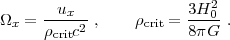
These are expressed as ratios to the critical energy
density required for flat space geometry
/ a, and
Ωm,
Ωr, and
Ωϕ are the present day
energy densities of matter, radiation, and a generic form of
dark energy ϕ.
10
These are expressed as ratios to the critical energy
density required for flat space geometry
 |
(4) |
At higher redshifts,
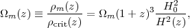 |
(5) |
where the second equality follows from the scaling ρm(z) = ρm,0 × (1 + z)3 and from the definition of ρcrit(z). In the formulation (3), the impact of curvature on expansion is expressed like that of a "dynamical" component with scaled energy density
 |
(6) |
with Ωk = 0 for a spatially flat universe. In a standard cold dark matter scenario, the matter density is the sum of the densities of CDM, baryons, and non-relativistic neutrinos, Ωm = Ωc + Ωb + Ων. In detail, one must beware that the neutrino energy density does not scale as (1 + z)3 at higher redshifts, when they are mildly relativistic, and that the clustering of neutrinos on small scales is suppressed by their residual thermal velocities.
There are some routes to direct measurement of H(z), most notably via BAO (see Section 4). For the most part, however, observations constrain H(z) indirectly by measuring the distance-redshift relation or the history of structure growth.
Hogg (1999) provides a compact and pedagogical summary of cosmological distance measures. The comoving line-of-sight distance to an object at redshift z is
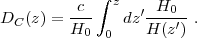 |
(7) |
Defining a dimensional (length-2) curvature parameter
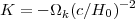 |
(8) |
allows us to write the comoving angular diameter distance, 11 relating an object's comoving size l to its angular size θ = l / DA, as
 |
(9) |
which applies for either sign of Ωk. 12 Noting that observations imply |Ωk| ≪ 1, we can Taylor expand equation (9) to write
 |
(10) |
which also yields the correct result DA = Dc for Ωk = 0. Note that positive space curvature (Ωtot > 1, K > 0) corresponds to negative Ωk, hence a smaller DA and larger angular size than in a flat universe. If uϕ(z) > uϕ,0 then the Hubble parameter at z > 0 is higher compared to a cosmological constant model with the same matter density and curvature (eq. 3), and distances to redshifts z > 0 are lower (eq. 9).
The luminosity distance relating an object's bolometric flux fbol to its bolometric luminosity Lbol is
 |
(11) |
The relation between luminosity and angular diameter distance is independent of cosmology, so the two measures contain the same information about H(z) and Ωk. For this reason, we will sometimes use D(z) to stand in generically for either of these transverse distance measures. Some methods (e.g., counts of galaxy clusters) effectively probe the comoving volume element that relates solid angle and redshift intervals to comoving volume Vc. We will denote this quantity
 |
(12) |
On large scales, the gravitational evolution of fluctuations in pressureless dark matter follows linear perturbation theory, according to which
 |
(13) |
where ti is an arbitrarily chosen initial time, the linear growth function G(t) obeys the differential equation
 |
(14) |
and the GR subscript denotes the fact that this equation applies in standard GR. 13 The solution to this equation can only be written in integral form for specific forms of H(z), and thus for specific dark energy models specifying uϕ(z). However, to a very good approximation the logarithmic growth rate of linear perturbations in GR is
 |
(15) |
where γ ≈ 0.55-0.6 depends only weakly on cosmological parameters (Peebles 1980, Lightman and Schechter 1990). Integrating this equation yields
 |
(16) |
where Ωm(z) is given by equation (5). Linder (2005) shows that equation (16) is accurate to better than 0.5% for a wide variety of dark energy models if one adopts
 |
(17) |
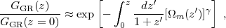
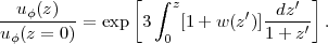
(see also Wang and Steinhardt 1998, Weinberg 2005, Amendola et al. 2005). While the full solution of equation (14) should be used for high accuracy calculations, equation (16) is useful for intuition and for approximate calculations. Note in particular that if uϕ(z) > uϕ,0 then, relative to a cosmological constant model, Ωm(z) ∝ H-2(z) is lower (eq. 5), so GGR(z) / GGR(z = 0) is higher — i.e., there has been less growth of structure between redshift z and the present day because matter has been a smaller fraction of the total density over that time. It is often useful to refer the growth factor not to its z = 0 value but to the value at some high redshift when, in typical models, dark energy is dynamically negligible and Ωm(z) ≈ 1. We will frequently use z = 9 as a reference epoch, in which case equation (16) becomes
 |
(18) |
In the limit Ωm(z) → 1, GGR(z) ∝ (1 + z)-1, i.e., the amplitude of linear fluctuations is proportional to a(t).
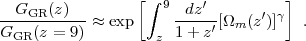
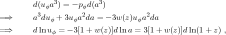
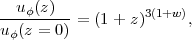
The properties of dark energy influence the observables — H(z), D(z), and G(z) — through the history of uϕ(z) / uϕ,0 in the Friedmann equation (3). This history is usually framed in terms of the value and evolution of the equation-of-state parameter w(z) = pϕ(z) / uϕ(z). Provided that the field ϕ is not transferring energy directly to or from other components (e.g., by decaying into dark matter), applying the first law of thermodynamics dU = -p dV to a comoving volume implies
 |
(19) (20) (21) |
where the last equality uses the definition a = (1 + z)-1. Integrating both sides implies
 |
(22) |
For a constant w independent of z we find
 |
(23) |
which yields the familiar results u ∝ (1 + z)3 for pressureless matter and u ∝ (1 + z)4 for radiation (w = +1/3), and which shows once again that a cosmological constant uϕ(z) = constant corresponds to w = -1.
The first obvious way to parameterize w(z) is with a Taylor expansion w(z) = w0 + w'z + ..., but this expansion becomes ill-behaved at high z. A more useful two-parameter model (Chevallier and Polarski 2001, Linder 2003a) is
 |
(24) |
in which the value of w evolves linearly with scale factor from w0 + wa at small a (high z) to w0 at z = 0. Observations usually provide the best constraint on w at some intermediate redshift, not at z = 0, so statistical errors on w0 and wa are highly correlated. This problem can be circumvented by recasting equation (24) into the equivalent form
 |
(25) |
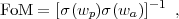
and choosing the "pivot" expansion factor ap so that the observational errors on wp and wa are uncorrelated (or at least weakly so). The value of the pivot redshift depends on what data sets are being considered, but in practice it is usually close to zp ≡ ap-1 -1 ≈ 0.4-0.5 (see Table 8). The best-fit wp is, approximately, the parameter of the constant-w model that would best reproduce the data. A cosmological constant would be statistically ruled out either if wp were inconsistent with -1 or if wa were inconsistent with zero. In practice, error bars on wa are generally much larger than error bars on wp, by a factor of 5-10. More generally, it is much more difficult to detect time dependence of w than to show w ≠ -1, typically requiring sub-percent measurements of observables even if w changes by order unity in an interval Δz < 1 at low redshift (Kujat et al. 2002). The DETF proposed a figure of merit (FoM) for dark energy programs based on the expected error ellipse in the w0 - wa plane (similar to the approach described by Huterer and Turner 2001). We will frequently refer to this DETF figure of merit, adopting the definition
 |
(26) |
and we will refer to dark energy models defined by equations (24) or (25) as "w0 - wa models."
An alternative parameterization approach is to approximate w(z) as a stepwise-constant function defined by its values in a number of discrete bins, perhaps with priors or constraints on the allowed values (e.g., -1 ≤ w(z) ≤ 1). For a given set of observations, this function can then be decomposed into orthogonal principal components (PCs), with the first PC being the one that is best constrained by the data, the second PC the next best constrained, and so forth (Huterer and Starkman 2003). Variants of this approach have been widely adopted in recent investigations (e.g., Albrecht and Bernstein 2007, Sarkar et al. 2008b, Mortonson et al. 2009b), including the report of the JDEM Figure-of-Merit Science Working Group (Albrecht et al. 2009). The PCA approach has the advantage of allowing quite general w(z) histories to be represented, though in practice only a few PCs can be constrained well; Linder and Huterer (2005) and de Putter and Linder (2008) have argued that the w0 - wa parameterization has equal power for practical purposes. We will use both characterizations for our forecasts in Section 8. For scalar field models, one can attempt to reconstruct the potential V(ϕ) instead of w(z) (Starobinsky 1998, Huterer and Turner 1999, Nakamura and Chiba 1999), an approach that we discuss briefly at the end of Section 8.3.4. Gott and Slepian (2011) emphasize that slowly rolling scalar field models generically predict 1 + w ≈ (1 + w0)H02 / H2(z) for |1 + w| ≪ 1, making the space of w(z) models, to leading order, one-dimensional, rather than the two-dimensional parameterization of w0 - wa. As a complement to parameterized models, one can attempt to construct non-parametric "null tests" for a cosmological constant or scalar field models (Sahni et al. 2008).
If w ≠ -1, then the dark energy density should display spatial inhomogeneities, but for simple scalar field models these inhomogeneities are strongly suppressed on scales below the horizon. More complicated models that have a sound speed (cs2 = δ p / δρ) much smaller than c allow fluctuations to grow on sub-horizon scales (e.g., Hu 1998, Erickson et al. 2002, Weller and Lewis 2003, DeDeo et al. 2003, Bean and Dori 2004). de Putter et al. (2010) provide a clear discussion of the background physics and observable consequences of dark energy inhomogeneities. In general these inhomogeneities are very difficult to detect, because their growth is significant only when w is far from -1 and cs ≪ c, and because the fluctuations in dark energy density are much smaller than those in dark matter. We will mostly ignore dark energy inhomogeneities in this article, though we return to the subject briefly in Section 7.8.
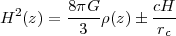
Our equations so far have assumed that GR is correct. The alternative to dark energy is to modify GR in a way that produces accelerated expansion. One of the best-studied examples is DGP gravity (Dvali et al. 2000), which posits a five-dimensional gravitational field equation that leads to a Friedmann equation
 |
(27) |
for a spatially flat, homogeneous universe confined to a (3 + 1)-dimensional brane. Above the "crossover scale" rc, which relates the five-dimensional and four-dimensional gravitational constants, the gravitational force law scales as r-3 instead of the usual r-2. Choosing the positive sign for the second term in equation (27) and setting rc ~ c / H0 leads to an initially decelerating universe that transitions to accelerating, and ultimately exponential, expansion. Other modifications to the gravitational action that replace the curvature scalar R by some function f(R) will modify the Friedmann equation in different ways, some of which can produce late-time acceleration (e.g., Capozziello and Fang 2002, Carroll et al. 2004). Alternatively, one can simply postulate a modified Friedmann equation without specifying a complete gravitational theory, e.g., by replacing ρ on the right hand side of H2 ∝ ρ with a parameterized function H2 ∝ g(ρ) (Freese and Lewis 2002, Freese 2005). Of course, there is no guarantee that such a function can in fact be derived from a self-consistent gravitational theory.
Using equations (3) and (22), one can express a modified Friedmann equation in terms of an effective time-dependent dark energy equation of state. In this review, we will use w(z) to parameterize the expansion histories of both dark energy and modified gravity theories. Given w(z), H(z) and D(z) generally follow from the same set of equations for both types of theories, so observations that only probe the geometry of the universe are incapable of distinguishing between the two possible explanations of cosmic acceleration. In addition to changing the Friedmann equation, however, a modified gravity model may alter the equation (14) that relates the growth of structure to the expansion history H(z). Therefore, one general approach to testing modified gravity explanations is to search for inconsistency between observables that probe H(z) or D(z) and observables that also probe the growth function G(z). Some methods effectively measure G(z) / G(z = 0), others measure G(z) relative to an amplitude anchored in the CMB, and others measure the logarithmic growth index γ of equation (15). For "generic" parameters that describe departures from GR-predicted growth, we will use a parameter G9 that characterizes an overall multiplicative offset of the growth factor and a parameter Δγ that characterizes a change in the fluctuation growth rate. We define these parameters in Section 2.4 below, following our review of CMB anisotropy and large scale structure. These parameters serve as useful diagnostics for deviations from GR, but they do not provide a complete description of the effects of modified gravity theories. In particular, it is also possible (see Section 7.7) that modified gravity will cause G(z) to be scale-dependent, or that it will alter the relation between gravitational lensing and non-relativistic mass tracers, or that it will reveal its presence through a high-precision test on solar system or terrestrial scales.
The above considerations lead to the following general strategy for probing the physics of cosmic acceleration: use observations to constrain the functions H(z), D(z), and G(z), and use these constraints in turn to constrain the history of w(z) for dark energy models and to test for inconsistencies that could point to a modified gravity explanation. For pure H(z) and D(z) measurements, the "nuisance parameters" in such a strategy are the values of Ωm and Ωk, in addition to parameters related directly to the observational method itself (e.g., the absolute luminosity of supernovae). Assuming a standard radiation content, the value of Ωϕ = 1 - Ωm - Ωr - Ωk is fixed once Ωm and Ωk are known. The effects of Ωm and Ωk are separable both from their different redshift dependence in the Friedmann equation (3) and from the influence of Ωk on transverse distances (eq. 9) via space curvature.
2.3. CMB Anisotropies and Large Scale Structure
CMB anisotropies have little direct constraining power on dark energy, but they play a critical role in cosmic acceleration studies because they often provide the strongest constraints on nuisance parameters such as Ωm, Ωk, and the high-redshift normalization of matter fluctuations. In particular, the amplitudes of the acoustic peaks in the CMB angular power spectrum depend sensitively (and differently) on the matter and baryon densities, and the locations of the peaks depend sensitively on spatial curvature. Using CMB constraints necessarily brings in additional nuisance parameters such as the spectral index ns and curvature d ns / dlnk of the scalar fluctuation spectrum, the amplitude and slope of the tensor (gravitational wave) fluctuation spectrum, the post-recombination electron-scattering optical depth τ, and the Hubble constant
 |
(28) |
However, some of these parameters are themselves relevant to cosmic acceleration studies, and current CMB measurements yield tight constraints even after marginalizing over many parameters (e.g., Komatsu et al. 2011). The strength of these constraints depends significantly on the adopted parameter space — for example, current CMB data provide tight constraints on h if one assumes a flat universe with a cosmological constant, but these constraints are much weaker if Ωk and w are free parameters.
CMB data are usually incorporated into dark energy constraints, or forecasts, by adding priors on parameters that are then marginalized over in the analysis. We will adopt this strategy in Section 8, using the level of precision forecast for the Planck satellite. However, it is worth noting some rules of thumb. For practical purposes, Planck data will give near-perfect determinations of Ωm h2 and Ωb h2 from the heights of the acoustic peaks, where the h2 dependence arises because it is the physical density that affects the acoustic features, not the density relative to the critical density. "Near-perfect" means that marginalizing over the expected uncertainties in Ωm h2 and Ωb h2 adds little to the error bars on dark energy parameters even from ambitious "Stage IV" experiments, relative to assuming that they are known perfectly. 14 Planck data will also give near-perfect determinations of the sound horizon at recombination rs(z*), which determines the physical scale of the acoustic peaks in the CMB and the scale of BAO in large scale structure (see Section 4.1). Since the angular scale of the acoustic peaks is precisely measured, Planck data should also yield a near-perfect determination of the angular diameter distance to the redshift of recombination, D* ≡ DA(z*), where z* ≈ 1091. Finally, the amplitude of CMB anisotropies gives a near-perfect determination (after marginalizing over the optical depth τ, which is constrained by polarization data) of the amplitude of matter fluctuations at z*, and thus throughout the era in which dark energy (or deviation from GR) is negligible. As emphasized by Hu (2005; an excellent source for more detailed discussion of CMB anisotropies in the context of dark energy constraints), these determinations all depend on the assumptions of a standard thermal and recombination history, but the CMB data themselves allow tests of these assumptions at the required level of accuracy. CMB data also allow tests of cosmic acceleration models via the integrated Sachs-Wolfe (ISW) effect, which we discuss briefly in Section 7.8.
If primordial matter fluctuations are Gaussian, as predicted by simple inflation models and supported by most observational investigations to date, then their statistical properties are fully specified by the power spectrum P(k) or its Fourier transform, the two-point correlation function ξ(r). Defining the Fourier transform of the density contrast 15
 |
(29) |
the power spectrum is defined by
 |
(30) |
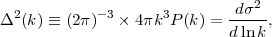
where δd3 is a 3-d Dirac-delta function and isotropy guarantees that P(k) is a function of k = |k| alone. The power spectrum has units of volume, and it is often more intuitive to discuss the dimensionless quantity
 |
(31) |
which is the contribution to the variance σ2 ≡ < δ2 > of the density contrast per logarithmic interval of k. The variance of the density field smoothed with a window Wr(r) of scale R is
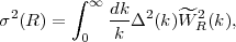 |
(32) |
where the Fourier transform of a top-hat window, Wr(r) = (4π R3/3)-1Θ(1-r / R), is
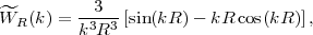 |
(33) |
and the Fourier transform of a Gaussian window, Wr(r) = (2π)-3/2 R-3 e-r2 / 2R2, is
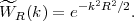 |
(34) |
The correlation function is
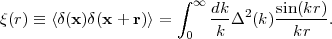 |
(35) |
In linear perturbation theory, the power spectrum amplitude is proportional to G2(z), and we will take Plin(k) to refer to the z = 0 normalization when the redshift is not otherwise specified:
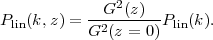 |
(36) |
We discuss the normalization of G(z) and Plin(k) more precisely in Section 2.4 below. The evolution of P(k) remains close to linear theory for scales k ≪ knl, where
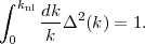 |
(37) |
For realistic power spectra, non-linear evolution on small scales does not feed back to alter the linear evolution on large scales (Peebles 1980, Shandarin and Melott 1990, Little et al. 1991). However, the shape of the power spectrum does change on scales approaching knl, in ways that can be calculated using N-body simulations (Heitmann et al. 2010) or several variants of cosmological perturbation theory (Carlson et al. 2009 and references therein). Non-linear evolution is a significant effect for weak lensing predictions and for the evolution of BAO, as we discuss in the corresponding sections below.
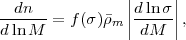
While there are many ways of characterizing the matter distribution in the non-linear regime, the two measures that matter the most for our purposes are the mass function and clustering bias of dark matter halos. There are several different algorithms for identifying halos in N-body simulations, all of them designed to pick out collapsed, gravitationally bound dark matter structures in approximate virial equilibrium. It is convenient to express the halo mass function in the form
 |
(38) |
where σ2 is the variance of the linear density field
smoothed with a top-hat filter of mass scale M = 4/3
π R3
 m
(eqs. 32 and 33). To a first approximation, the function
f(σ) is universal,
and the effects of power spectrum shape, redshift (and thus power
spectrum amplitude), and background cosmological model
(e.g., Ωm and
ΩΛ) enter only through
determining |dlnσ / dM| and
m.
The state-of-the-art numerical investigation is that of
Tinker et
al. (2008),
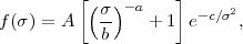
who fit a large number of N-body simulation results with the functional
form
m
(eqs. 32 and 33). To a first approximation, the function
f(σ) is universal,
and the effects of power spectrum shape, redshift (and thus power
spectrum amplitude), and background cosmological model
(e.g., Ωm and
ΩΛ) enter only through
determining |dlnσ / dM| and
m.
The state-of-the-art numerical investigation is that of
Tinker et
al. (2008),
who fit a large number of N-body simulation results with the functional
form
 |
(39) |
finding best-fit values A = 0.186, a = 1.47, b =
2.57, c = 1.19
for z = 0 halos, defined to be spherical regions centered on density
peaks enclosing a mean interior overdensity of 200 times the
cosmic mean density
m.
(Different halo mass definitions lead to different coefficients.)
A similar functional form was justified on analytic grounds by
Sheth and Tormen
(1999),
following a chain of argument that ultimately traces back to
Press and Schechter
(1974)
and
Bond et al. (1991).
Discussions of the halo population frequently refer to the
characteristic mass scale M*, defined by
 |
(40) |
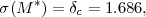
which sets the location of the exponential cutoff in the Press-Schechter mass function. Here δc is the linear theory overdensity at which a spherically symmetric perturbation would collapse. 16
In detail, Tinker et al. (2008) find that f(σ) depends on redshift at the 10-20% level, probably because of the dependence of halo mass profiles on Ωm(z). At overdensities of ~ 200, the baryon fraction in group and cluster mass halos (M > 1013 M⊙) is expected to be close to the cosmic mean ratio Ωb / Ωm, but gas pressure, dissipation, and feedback from star formation and AGN can alter this fraction and change baryon density profiles relative to dark matter profiles. We discuss these issues further in Section 6.
Massive halos are more strongly clustered than the underlying matter distribution because they form near high peaks of the initial density field, which arise more frequently in regions where the background density is high (Kaiser 1984, Bardeen et al. 1986). On large scales, the correlation function of halos of mass M is a scale-independent multiple of the matter correlation function ξhh(r) = bh2(M) ξmm(r). The halo-mass cross-correlation in this regime is ξhm(r) = bh(M) ξmm(r), and similar scalings (bh2 and bh) hold for the halo power spectrum and halo-mass cross spectrum at low k. Analytic arguments suggest a bias factor (Cole and Kaiser 1989, Mo and White 1996)
 |
(41) |
There have been numerous refinements to this formula based on analytic models and numerical calibrations. The state-of-the-art numerical study is that of Tinker et al. (2010).
Galaxies reside in dark matter halos, and they, too, are biased tracers of the underlying matter distribution. Here one must allow for the fact that different kinds of galaxies reside in different mass halos and that massive halos host multiple galaxies. More massive or more luminous galaxies are more strongly clustered because they reside in more massive halos that have higher bh(M). At low redshift, the large scale bias factor is bg ≤ 1 for galaxies below the characteristic cutoff L* of the Schechter (1976) luminosity function, but it rises sharply at higher luminosities (Norberg et al. 2001, Zehavi et al. 2005, Zehavi et al. 2011).
For a galaxy sample defined by a threshold Lmin in optical or near-IR luminosity (or stellar mass), theoretical models and empirical studies (too numerous to list comprehensively, but our summary here is especially influenced by Kravtsov et al. 2004, Conroy et al. 2006, Zehavi et al. 2011) suggest the following approximate model. The minimum host halo mass is the one for which the comoving space density n(Mmin) of halos above Mmin matches the space density n(Lmin) of galaxies above the luminosity threshold. Each halo above Mmin hosts one central galaxy, and in addition each such halo hosts a mean number of satellite galaxies < Nsat> = (M - Mmin) / 15Mmin, with the actual number of satellites drawn from a Poisson distribution with this mean. 17 The large scale galaxy bias factor bg is the average bias factor bh(M) of halos above Mmin, with the average weighted by the product of the halo space density and the average number of galaxies per halo. In addition to increasing bg by giving more weight to high mass halos, satellite galaxies contribute to clustering on small scales, where pairs or groups of galaxies reside in a single halo (Seljak 2000, Scoccimarro et al. 2001, Berlind and Weinberg 2002). In detail, at high luminosities one must allow for scatter between galaxy luminosity and halo mass, which reduces the bias below that of the sharp threshold model described above. Furthermore, selecting galaxies by color or spectral type alters the relative fractions of central and satellite galaxies; redder, more passive galaxies are more strongly clustered because a larger fraction of them are satellites, and the reverse holds for bluer galaxies with active star formation. Thus each class of galaxies has its own halo occupation distribution (HOD), which describes the probability P(N|M) of finding N galaxies in a halo of mass M and specifies any relative bias of galaxies and dark matter within halos.
On large scales, where bg2
Δlin2(k,z) ≪ 1,
the galaxy power
spectrum should have the same shape as the linear matter power
spectrum, Pgg(k, z) =
bg2 Plin(k,
z). However, scale-dependence
of bias at the 10-20% level can persist to quite low k, especially
for luminous, highly biased galaxy populations,
and the effective "shot noise" contribution to
Pgg(k) can
differ from the naive 1 /
 g
term expected for
Poisson statistics
(Yoo et al. 2009).
Combinations of CMB power spectrum measurements with galaxy power
spectrum measurements can yield tighter cosmological parameter
constraints than either one in isolation (e.g.,
Cole et al. 2005,
Reid et al. 2010).
In particular, this combination provides greater leverage on
the Hubble constant h, since CMB-constrained models predict
galaxy clustering in Mpc while galaxy redshift surveys measure
distances in h-1 Mpc (or, equivalently, in km
s-1).
g
term expected for
Poisson statistics
(Yoo et al. 2009).
Combinations of CMB power spectrum measurements with galaxy power
spectrum measurements can yield tighter cosmological parameter
constraints than either one in isolation (e.g.,
Cole et al. 2005,
Reid et al. 2010).
In particular, this combination provides greater leverage on
the Hubble constant h, since CMB-constrained models predict
galaxy clustering in Mpc while galaxy redshift surveys measure
distances in h-1 Mpc (or, equivalently, in km
s-1).
Another complicating factor in galaxy clustering measurements is redshift-space distortion (Kaiser 1987; see Hamilton 1998 for a comprehensive review), which arises because galaxy redshifts measure a combination of distance and peculiar velocity rather than true distance. On small scales, velocity dispersions in collapsed objects stretch structures along the line of sight. On large scales, coherent inflow to overdense regions compresses them in the line-of-sight direction, and coherent outflow from underdense regions stretches them along the line of sight. In linear perturbation theory, the divergence of the peculiar velocity field is related to the density contrast field by
 |
(42) |
with γ defined by equation (15). The galaxy redshift-space power spectrum in linear theory is anisotropic, depending on the angle θ between the wavevector k and the observer's line of sight as
 |
(43) |
where P(k) is the real-space matter power spectrum, μ ≡ cosθ, and f(z) ≈ [Ωm(z)]γ is the logarithmic growth rate (eq. 15). The strength of the anisotropy depends on the ratio β ≡ f(z) / bg; because linear bias amplifies galaxy clustering isotropically, more strongly biased galaxies exhibit weaker redshift-space distortion. A variety of non-linear effects, most notably the small scale dispersion and its correlation with large scale density, mean that equation (43) is rarely an adequate approximation in practice, even on quite large scales (Cole et al. 1994, Scoccimarro 2004). In the galaxy correlation function, one can remove the effects of redshift-space distortion straightforwardly by projection, counting galaxy pairs as a function of projected separation rather than 3-d redshift-space separation. For the power spectrum, one can correct for redshift-space distortion, but the analysis is more model-dependent (see, e.g., Tegmark et al. 2004). However, redshift-space distortion can be an asset as well as a nuisance, since it provides a route to measuring dlnG / dlna. We will discuss this idea at some length in Section 7.2, as it is emerging as a powerful route to measuring the expansion history and testing GR growth predictions.
2.4. Parameter Dependences and CMB Constraints
Figure 1 illustrates the four statistics discussed above: the CMB temperature angular power spectrum, the matter variance Δlin2(k) computed from the linear theory power spectrum at z = 0, the z = 0 halo mass function computed from equations (38) and (39), and the halo bias factor computed from equation (6) of Tinker et al. (2010) for overdensity 200 halos (relative to the mean matter density). Curves in the main panels show a fiducial model with the likelihood-weighted mean parameters for the seven-year WMAP CMB measurements (hereafter WMAP7; Larson et al. 2011) assuming a flat universe with a cosmological constant: Ωc = 0.222, Ωb = 0.045, ΩΛ = 0.733, h = 0.71, ns = 0.963, τ = 0.088, and primordial power spectrum amplitude As(k = 0.002 Mpc-1) = 2.43 × 10⁻⁹. (These parameters also assume no tensor fluctuations and dns / dlnk = 0.) The CMB power spectrum shows the familiar pattern of acoustic peaks, with the angular scale of the first peak corresponding approximately to the sound horizon at recombination divided by the angular diameter distance to the last scattering surface. The matter variance Δlin2(k) shows a slow change of slope starting at k ≈ 0.02 h Mpc-1, corresponding to the horizon scale at matter-radiation equality, and low amplitude wiggles at smaller scales produced by BAO. The halo mass function has an approximate power-law form at low masses changing slowly to an exponential cutoff for M ≫ M* = 3 × 10¹² h-1 M⊙. The bh(M) relation is roughly flat for M ≲ 5 M* before rising steeply at higher masses. The h-dependences used for k, dn / dlnM, and M reflect the dependences that typically arise when distances are estimated from redshifts and thus scale as h-1.
 |
Figure 1. CMB angular power spectrum (upper left), variance of matter fluctuations (upper right), halo mass function (lower left), and halo bias factor (lower right). Solid curves in the main panels show predictions of the fiducial ΛCDM panel listed in Table 1. Curves in the lower panels show the fractional changes in these statistics induced by changing 1 + w to ± 0.1 or Ωk to ± 0.01 (see legend). For each parameter change, we keep Ωm h2, Ωb h2, and D* fixed by adjusting Ωm, Ωb, and h (see Table 1). These compensating changes keep deviations in the CMB spectrum minimal, much smaller than the cosmic variance errors indicated by the shaded region. |
In the lower panels, we show the fractional change in these statistics that arises when changing 1 + w from 0 to ± 0.1 and when changing Ωk from 0 to ± 0.01. With any parameter variation, there is the crucial question of what one holds fixed. For this figure, we have held fixed the parameter combinations that have the strongest impact on the CMB power spectrum: Ωm h2 and Ωb h2, which determine the heights of the acoustic peaks and the physical scale of the sound horizon, and D* = DA(z*), which maps the physical scale of the peaks into the angular scale. We satisfy these constraints by allowing h and Ωm to vary, maintaining Ωk = 0 for the w-variations and w = -1 for the Ωk-variations, with ns, As, and τ fixed to the fiducial model values. The parameter values for these variant models appear in Table 1.
| w | Ωk | Ωc | Ωb | Ωϕ | h | σ8 |
| -1.0 | 0.00 | 0.222 | 0.045 | 0.733 | 0.710 | 0.806 |
| -0.9 | 0.00 | 0.246 | 0.050 | 0.704 | 0.675 | 0.774 |
| -1.1 | 0.00 | 0.201 | 0.041 | 0.758 | 0.746 | 0.837 |
| -1.0 | 0.01 | 0.186 | 0.038 | 0.766 | 0.776 | 0.809 |
| -1.0 | -0.01 | 0.256 | 0.052 | 0.702 | 0.661 | 0.802 |
| All models have ns = 0.963, τ = 0.088, As(k = 0.002 Mpc-1) = 2.43W 10-9. In addition, all models have the same values Ωm h2, Ωb h2, and distance to the last scattering surface D*, so they produce nearly indistinguishable CMB power spectra. | ||||||
From the CMB panel, we can see that the changes in the angular power spectrum induced by these parameter variations are small compared to the cosmic variance error at every l, since we have fixed the parameter combinations that mostly determine the CMB spectrum. 18 The changes are coherent, of course, but even considering model fits to the entire CMB spectrum the w changes would be undetectable at the level of errors forecast for Planck, while the Ωk = ± 0.01 models would be distinguishable from the fiducial model at about 1.5σ. The impact of these parameter changes must instead be sought in other statistics at much lower redshifts. Changes to the matter variance are ~ 5% at small scales, growing to ~ 20% at large scales, with oscillations that reflect the shift in the BAO scale. Fractional changes to the halo space density at fixed mass can be much larger, especially at high masses where the halo mass function is steep. We caution, however, that the fractional change in mass at fixed abundance is significantly smaller, a point that we emphasize in Section 6. The impact of a change in w reverses sign at M ≈ 6 × 10¹⁴ h-1 M⊙ ≈ 200 M*, where the mass function begins to drop sharply. Changes in bias factor at fixed mass are ~ 5% at high masses and smaller at low masses.
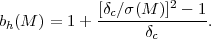
Figure 2 shows the redshift evolution and parameter sensitivity of the Hubble parameter (eq. 3) and the comoving angular diameter distance (eq. 9), for the same fiducial model and parameter variations used in Figure 1. The upper panels show H(z) and DA(z) in absolute units, while the lower panels plot them in h-1 Gpc units. BAO studies measure in absolute units, but supernova studies effectively measure hDA(z) because they are calibrated in the local Hubble flow. Equivalently, supernova distances are determined in h-1 Mpc rather than Mpc. 19 Weak lensing predictions depend on distance ratios rather than absolute distances, so in practice they also constrain hDA(z) rather than absolute DA(z).
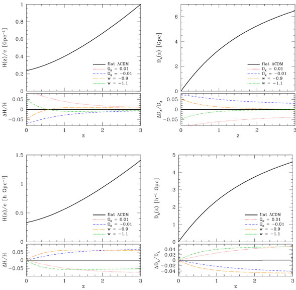 |
Figure 2. Evolution of the Hubble parameter (left) and the comoving angular diameter distance (right) for the fiducial ΛCDM model and for the variant models shown in Figure 1. Upper panels are in absolute units, relevant for BAO, while lower panels show distances in h-1 Gpc, relevant for supernovae or weak lensing. |
In absolute units, model predictions diverge most strongly at z = 0, and the impact of Ωk = ± 0.01 is larger than the impact of 1 + w = ± 0.1. The impact of the w change on H(z) reverses sign at z ≈ 0.6, a consequence of our CMB normalization. Changing w to -0.9 would on its own reduce the distance to z*, and H0 must therefore be lowered to keep D* fixed. However, with Ωm h2 fixed, lower H0 implies a higher Ωm, which raises the ratio H(z) / H0, and at high redshift this effect wins out over the lower H0. At z > 2, DA(z) remains sensitive to Ωk but is insensitive to w, while the sensitivity of H(z) to w is roughly flat for 1 < z < 3. In h-1 Mpc units, models converge at z = 0 by definition, and the impact of 1 + w = ± 0.1 is generally larger than the impact of Ωk = ± 0.01. The sensitivity of hDA(z) to parameter changes increases monotonically with increasing redshift, growing rapidly until z = 0.5 and flattening beyond z = 1.
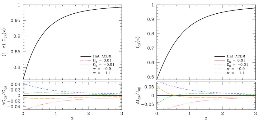 |
Figure 3. Evolution of the linear growth factor G(z) and growth rate f(z) for the models shown in Figure 2, assuming GR. The scaling in the left panel removes the (1 + z) evolution that would arise in an Ωm = 1 universe and normalizes GGR(z) to one at z = 9. |
For structure growth, the issues of normalization are more subtle. The normalization of the matter power spectrum is known better from CMB anisotropy at z* than it is from local measurements at z = 0, and this will be still more true in the Planck era. It therefore makes sense to anchor the normalization in the CMB, even though the value at z = 0 then depends on cosmological parameters. Figure 3 (left panel) plots (1 + z)GGR(z), where GGR(z) obeys equation (14) and is normalized to unity at z = 9. In most models, dark energy is dynamically negligible at z > 9, making the growth from the CMB era up to that epoch independent of dark energy. In an Ωm = 1 universe, GGR(z) ∝ (1 + z)-1, so the plotted ratio falls below unity when Ωm(z) starts to fall below one. For Ωk = 0.01, Ωm(z) is below that in our fiducial model (see eqs. 3 and 5) both because of the Ωk term in the Friedmann equation and because we lower Ωm(z = 0) from 0.27 to 0.22 to keep D* fixed, thus depressing GGR(z) increasingly towards lower z. For w = -0.9, however, the depression of Ωm(z) / Ωm(z = 0) from the Friedmann equation is countered by the higher value of Ωm(z = 0) = 0.30 adopted to fix D*, so the depression of GGR(z) is smaller, and it actually recovers towards the fiducial value as z approaches zero. The effects on the growth rate f(z) (right panel) are similar but stronger, with our adopted parameter changes producing larger deviations from the fiducial model and the influence of w actually reversing sign at z < 0.5.
 |
Figure 4. Evolution of the matter fluctuation amplitude for the models shown in Figure 3, characterized by the rms linear fluctuation in comoving spheres of radius 8 h-1 Mpc (left) or 11 Mpc (right). All models are normalized to the WMAP7 CMB fluctuation amplitude. |
In practice, observations do not probe the growth factor itself but the amplitude of matter clustering, and in this case we must also account for the changing relation between the CMB power spectrum and the matter clustering normalization. The left panel of Figure 4 plots σ8(z) × (1 + z), where σ8(z) is the rms linear theory density contrast in a sphere of comoving radius 8 h-1 Mpc (eqs. 32 and 33). The right panel instead plots σ11,abs(z) × (1 + z), where σ11,abs refers to a sphere of radius 11 Mpc (equivalent to σ8 for h = 0.727). At high redshift these curves go flat as Ωm(z) approaches one and the growth rate approaches GGR(z) ∝ (1 + z)-1. In the CMB-matched models considered here, the impact of w or Ωk changes is complex, since changing these parameters alters the best-fit values of Ωm and h as well as changing the growth factor directly through equation (16). The values of σ8(z) change by 4-5% at all z for 1 + w = ± 0.1, but these changes mostly track the changes in h. In absolute units, the changes to σ11,abs(z) are ≲ 1%, tracking (by definition) the changes in GGR(z) shown in Figure 3. For Ωk = ± 0.01, σ8(z) changes by 4-5% at high z but converges nearly to the fiducial value at z = 0, while σ11,abs(z) shows only 1% differences at high z but diverges at low z.
All of these models have the WMAP7 (Larson et al. 2011) normalization of the power spectrum of inflationary fluctuations, As = 2.43 × 10⁻⁹ at comoving scale k = 0.002 Mpc-1 at z = z* = 1091. The primary uncertainty in this normalization is the degeneracy with the electron optical depth τ, since late-time scattering suppresses the amplitude of the primary CMB anisotropies by a factor e-τ on the scales that determine the normalization. The WMAP7 constraints are τ = 0.088 ± 0.015 (1σ), so the associated uncertainty in the matter fluctuation amplitude is 1.5%. (Recall that the power spectrum amplitude is ∝ σ82, so its fractional error is a factor of two larger.) For Planck, Holder et al. (2003) estimate uncertainty στ = 0.01 allowing for complex reionization history, and we use this value in our own forecasts. While there have been some changes in the situation since then (the polarized foregrounds at large scales are worse than anticipated, and τ is lower than the central value from the first-year WMAP results), this expectation seems broadly consistent with more recent studies (e.g., Mortonson and Hu 2008, Colombo and Pierpaoli 2009). 20 This will likely be the limiting factor for comparison of high-redshift (CMB) measurements with low-redshift (e.g., WL) measurements of the growth of structure (as opposed to measurements of evolution within the observed low-z range), unless other probes of reionization such as 21 cm provide constraints on the reionization history (see Section 5.9 for further discussion).
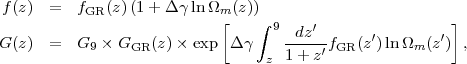
Following Albrecht et al. (2009), we parameterize departures from the GR growth rate by a change Δγ of the growth index (eq. 15) and by an overall amplitude shift G9 that is the ratio of the matter fluctuation amplitude at z = 9 to the value that would be predicted by GR given the same cosmological parameters and w(z) history. 21 Some caution is required in defining Δγ, since equations (15)-(17) are not exact, and their inaccuracies should not be defined as failures of GR! For precise calculations, therefore, we adopt the Albrecht et al. (2009) expressions for growth factor evolution:
 |
(44) (45) |
where GGR(z) and fGR(z) follow the (exact) solution to equation (14).
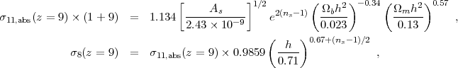
For practical purposes, one can use our definition of growth parameters to calculate the normalized linear theory matter power spectrum at redshift z, given an assumed set of cosmological parameter values and a w(z) history, as follows. First, use CAMB (Lewis et al. 2000) or some similar program to compute the normalized linear matter power spectrum at z = 9. Then multiply the power spectrum by G2(z) / GGR2(z = 9), with G(z) given by equation (45) and GGR(z) / GGR(z = 9) given by the exact solution to equation (14), or by the approximate integral solution (18), computing H(z) and Ωm(z) from equations (3) and (5) given the cosmological parameters and w(z). For reference, we note that CAMB normalization with WMAP7 data yields, for a flat ΛCDM model,
 |
(46) (47) |
where the primordial amplitude As is defined at comoving wavenumber k = 0.002 Mpc-1. This formula, similar to that in Hu and Jain (2004), is found by varying the parameters in CAMB calculations around the WMAP7 mean values one at a time to evaluate logarithmic derivatives; spot checks indicate that it is accurate to 0.2% over the 2σ range of the WMAP7 errors, and for the range of w and Ωk variations in Table 1. For models other than flat ΛCDM, one can use this formula to get σ8(z = 9) in GR, assuming that the effect of dark energy at z > 9 is negligible, then multiply by G(z) / GGR(z = 9) to get σ8(z).
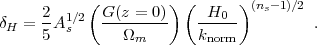
For an analytic power spectrum, one can use the approximate formula in equation (25) of Eisenstein and Hu 1999, which includes suppression of small scale power by baryonic effects but does not incorporate BAO. This paper defines the power spectrum normalization in terms of a parameter δh, related to our growth factor and normalization As by
 |
(48) |
Using the appropriate values for our fiducial WMAP7 flat ΛCDM model [G(z = 0) = 0.76, Ωm = 0.267, As = 2.43 × 10⁻⁹ at knorm = 0.002 Mpc-1, h = 0.71, ns = 0.963] with this definition of δh, the Eisenstein and Hu (1999) formula agrees with the result from CAMB to 2% or better except at the BAO scales, where deviations are up to 10%. One can also use this normalization for the more complex (but still analytic) formulae of Eisenstein and Hu (1998), which do include BAO. We caution that other papers and books (e.g., Dodelson 2003) have different definitions of δh.
There are, of course, degeneracies between the modified gravity parameters G9 and Δγ and the w(z) history, since both affect structure growth. However, if w(z) is pinned down well by D(z) and H(z) measurements, then measurements of matter clustering can be used to constrain G9 and Δγ. The clustering amplitude at a single redshift yields a degenerate combination of these two parameters, but measurements at multiple redshifts or direct measurements of the growth rate via redshift-space distortions can separate them in principle. Of course, there is no guarantee that a modified gravity prediction can be adequately described by G9 and a constant Δγ, and one might more generally consider (in eq. 45), for example, a functional history γ(z) analogous to w(z), or a direct multiplicative change to the growth rate dlnG / dlna rather than a change of the growth index γ. However, any constraints inconsistent with G9 = 1, Δγ = 0 after marginalizing over w(z) and cosmological parameters would be suggestive evidence for a breakdown of GR. Even if the measurements themselves are convincing, one must be cautious in the interpretation, since apparent discrepancies could arise from w(z) histories outside the families considered in marginalization or from other violations of the underlying assumptions. To give two examples, "early dark energy" that is dynamically significant at high redshift could cause an apparent G9 < 1, and decay of dark matter into dark energy could cause an apparent Δγ < 0 because the value of Ωm(z) / Ωm(z = 0) would be higher than in the standard picture. In Section 7.7 we discuss other potential signatures of modified gravity, such as scale-dependent growth, discrepancy between masses inferred from lensing and from non-relativistic tracers, and different accelerations in low and high density environments, and we mention other parameterizations that have been used to describe modified gravity models.
While they are not a substitute for full calculations, we find the use of CMB-normalized models like those in this section to be a valuable source of intuition for understanding the impact of distance or structure growth measurements in a (realistic) situation where CMB anisotropies impose tight parameter constraints. To make construction of such model sets easy, we note that for small changes |1 + w| ≲ 0.1 and |Ωk| ≲ 0.01, the changes to h required to keep D* fixed are well approximated by
 |
(49) |
The changes to Ωm and Ωb are then trivially found by fixing Ωm h2 and Ωb h2 to their fiducial model values, and the dark energy density follows from Ωϕ = 1 - Ωm - Ωk - Ωr. The value of σ11,abs(z = 9) is unchanged because Ωm h2 and Ωb h2 are fixed, while the value of σ8(z = 9) follows from equation (46) with the revised Hubble parameter. To compute power spectrum normalizations at other redshifts one uses equation (18) with the new Ωm(z) implied by equations (3) and (5). The changes to the normalization at z = 0 are approximately
 |
(50) |
The coefficients in equations (49) and (50) are chosen to reproduce the values in Table 1; at smaller |1 + w| or |Ωk| the best coefficients might be slightly different, but the changes themselves would be smaller.
We conclude our "background" material with a short overview of the methods we will describe in detail over the next four sections.
Observations show that Type Ia supernovae have a peak luminosity that is tightly correlated with the shape of their light curves — supernovae that rise and fall more slowly have higher peak luminosity. The intrinsic dispersion around this relation is only about 0.12 mag, allowing each well observed supernova to provide an estimated distance with a 1σ uncertainty of about 6%. Surveys that detect tens or hundreds of Type Ia supernovae and measure their light curves and redshifts can therefore measure the distance-redshift relation D(z) with high precision. Because the supernova luminosity is calibrated mainly by local observations of systems whose distances are inferred from their redshifts, supernova surveys effectively measure D(z) in units of h-1 Mpc, not in absolute units independent of H0.
Baryon acoustic oscillations provide an entirely independent way of measuring cosmic distance. Sound waves propagating before recombination imprint a characteristic scale on matter clustering, which appears as a local enhancement in the correlation funtion at r ≈ 150 Mpc. Imaging surveys can detect this feature in the angular clustering of galaxies in bins of photometric redshift, yielding the angular diameter distance D(zphot). A spectroscopic survey over the same volume resolves the BAO feature in the line-of-sight direction and thereby yields a more precise DA(z) measurement. Furthermore, measuring the BAO scale in velocity separation allows a direct determination of H(z). Other tracers of the matter distribution can also be used to measure BAO. Because the BAO scale is known in absolute units (based on straightforward physical calculation and parameter values well measured from the CMB), the BAO method measures D(z) in absolute units — Mpc not h-1 Mpc — so BAO and supernova measurements to the same redshift carry different information.
The shapes of distant galaxies are distorted by the weak gravitational lensing from matter fluctuations along the line of sight. The typical distortion is only ~ 0.5%, much smaller than the ~ 30% dispersion of intrinsic galaxy ellipticities, but by measuring the correlation of ellipticities as a function of angular separation, averaged over many galaxy pairs, one can infer the power spectrum of the matter fluctuations producing the lensing. Alternatively, one can measure the average elongation of background, lensed galaxies as a function of projected separation from foreground lensing galaxies to infer the galaxy-mass correlation function of the foreground sample, which can be combined with measurements of galaxy clustering to infer the matter clustering. By measuring the projected matter power spectrum for background galaxy samples at different z, weak lensing can constrain the growth function G(z). However, the strength of lensing also depends on distances to the sources and lenses, so in practice the weak lensing method constrains combinations of G(z) and D(z).
Clusters of galaxies trace the high end of the halo mass function, typically M ≥ 1014 M⊙. Observationally, one measures the number of clusters as a function of a mass proxy, which directly constrains dn / (dlnM dVc), where dn / dlnM is the halo mass function (eq. 38) and dVc is the comoving volume element at the redshift of interest (eq. 12). The mass function at high M is sensitive to the amplitude of matter fluctuations, and therefore to G(z), though this information is mixed with that in the cosmology dependence of the volume element dVc ∝ DA2 H-1. Clusters can be identified in optical/near-IR surveys that find peaks in the galaxy distribution and measure their richness, in wide-area X-ray surveys that find extended sources and measure their X-ray luminosity and temperature, or in Sunyaev-Zel'dovich (SZ) surveys that find localized CMB decrements and measure their depth. The critical step in any cluster cosmology investigation is calibrating the relation between halo mass and the survey's cluster observable — richness, luminosity, temperature, SZ decrement — so that the mass function can be inferred from (or constrained by) the distribution of observables. We will argue in Section 6 that the most reliable route to such calibration is via weak lensing, making wide-area optical or near-IR imaging a necessary component of any high-precision cosmic acceleration studies with clusters.
Several of the "alternative" methods described in Section 7 may ultimately play an important role in pinning down the origin of cosmic acceleration, even given the high precision expected from Stage IV supernova, BAO, weak lensing, and cluster surveys. In some cases, such as redshift-space distortions, these alternatives are automatically enabled by the same surveys conducted for BAO or weak lensing. In other cases, such as direct measurement of H0, the required observational programs are different in character.
10 We will refer to values of these parameters at z ≠ 0 as Ωm(z), Ωϕ(z), etc. For other quantities (e.g., H0), we use subscripts 0 to denote values at z = 0. When we assume a cosmological constant, we will replace Ωϕ by ΩΛ.
11 Note that Hogg (1999) refers to this quantity as the comoving transverse distance and uses DA to denote the quantity relating physical size to angular size. Back.
12 Recall that sin(ix) = isinh(x). Back.
13 This equation applies on scales much smaller than the horizon. On scales close to the horizon one must pay careful attention to gauge definitions. Yoo (2009) and Yoo et al. (2009) provide a unified and comprehensive discussion of the multiple GR effects that influence observable large scale structure on scales approaching the horizon. Back.
14 However, the effects of Planck-level CMB uncertainties are not completely negligible. For the fiducial Stage IV program discussed in Section 8, fixing Ωm h2 and Ωb h2 instead of marginalizing increases the DETF FoM from 664 to 876. Back.
15 A variety of Fourier conventions float around the cosmology literature. Here we adopt the same Fourier conventions and definitions as Dodelson (2003). Back.
16 See Gunn and Gott (1972), but note that their argument must be corrected to growing mode initial conditions, as is done in standard textbook treatments. The value δc = 1.686 is derived for Ωm = 1, but the cosmology dependence is weak. Back.
17 To make the model more accurate, one should adjust Mmin iteratively so that the total space density of galaxies, central+satellite, matches the observed n(Lmin), but this is usually a modest correction because the typical fraction of galaxies that are satellites is 5-20%. Back.
18 The CMB cosmic variance error is ΔlnClTT = [(2l + 1)/2]-1/2, determined simply by the number of modes on the sky at each angular scale l. Back.
19 To be more precise, studies of supernovae at redshifts z1 and z2 yield the distance ratio D(z2) / D(z1). When the z1 population is local, in the sense that inferred distances have negligible cosmology dependence except for the H0-1 scaling, then one gets the distance D(z2) in h-1 Mpc. Back.
20 For example, Colombo and Pierpaoli (2009) find στ ~ 0.006, albeit under somewhat optimistic assumptions regarding foregrounds and sky cuts. Back.
21 Albrecht et al. (2009) denote this quantity G0 instead of G9, but we have reserved subscript-0 to refer to z = 0 quantities. Back.