


The baryon acoustic oscillation method relies on the imprint left by sound waves in the early universe to provide a feature of known size in the late-time clustering of matter and galaxies. By measuring this acoustic scale at a variety of redshifts, one can infer DA(z) and H(z). The acoustic length scale can be computed as the comoving distance that the sound waves could travel from the Big Bang until recombination at z = z* (see descriptions by Hu and Sugiyama 1996, Eisenstein and Hu 1998). This is a simple integral
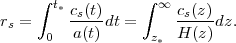 |
(52) |
The behavior of H(z) at z > z* depends on the ratio of the matter density to radiation density; in simple cosmologies, the radiation sector (photons and neutrinos) is fixed and the ratio is proportional to Ωm h2. The sound speed depends on the ratio of radiation pressure to the energy density of the baryon-photon fluid, determined by the baryon-to-photon ratio, which is proportional to Ωb h2. Both the matter-to-radiation ratio and the baryon-to-photon ratio are well measured by the relative heights of the acoustic peaks in the CMB anisotropy power spectrum. Analyses of WMAP data in the usual ΛCDM cosmological models gives a 1.1% inference of the acoustic scale rs (Jarosik et al. 2011); Planck is expected to shrink this error bar to 0.25%. Note that the acoustic scale is determined in absolute units, Mpc not h-1 Mpc.
The acoustic scale is large, about 150 Mpc comoving, because primordial sound waves travel at relativistic speed, maxing out at c / √3 at early times when the baryon density is negligible compared to radiation density. The large size of the acoustic scale protects this clustering feature from non-linear structure formation in the low-redshift universe. As discussed below, both cosmological perturbation theory and numerical simulations argue that the scale of the acoustic feature is stable to better than 1% accuracy, making it an excellent standard ruler. The BAO method measures the cosmic distance scale using this ruler. Separations along the line of sight correspond to differences in redshift that depend on the Hubble parameter H(z)rs. Separations transverse to the line of sight correspond to differences in angle that depend on the angular diameter distance DA(z) / rs.
The challenge of the BAO method is primarily statistical: because this is a weak signal at a large scale, one needs to map enormous volumes of the universe to detect the BAO and obtain a precise distance measurement. Galaxy redshift surveys allow us to make these large three-dimensional maps of the universe, although we will discuss other methods as well.
At low redshift (z ≲ 0.5), the BAO method strongly complements SN measurements because BAO provides an absolute distance scale and a strong connection to the CMB acoustic peaks from z = 1000, while SN allow more precise measurements of relative distances and thus offer a more fine-grained view of the distance-redshift relation. At higher redshift (z ≳ 0.5), the large cosmic volume and the direct access to H(z) make the BAO method an exceptionally powerful probe of dark energy and cosmic geometry.
4.2. The Current State of Play
 |
Figure 8. (Left) The current BAO distance-redshift relation. Individual measurements are of the quantity DV(z) / rs. We have multiplied by the rs of the fiducial ΛCDM model to yield a distance; the sound horizon is predicted to 1.1% from WMAP7. In increasing redshift, data points are from the 6dFGS (Beutler et al. 2011), SDSS-II (Padmanabhan et al. 2012, Xu et al. 2012b), BOSS (Anderson et al. 2012), and WiggleZ (Blake et al. 2011d). The WiggleZ paper also quotes correlated results from multiple redshift bins, but we have chosen to plot only a single combined data point for each survey so that the measurement errors are uncorrelated. As described in the text, for a fixed choice of w(z) and Ωk, CMB data allows a prediction for DV(z) / rs. The flat ΛCDM prediction from the best-fit WMAP7 model is the black line, and the grey region shows the 1σ WMAP7 range. This is not a fit to the data, but rather the vanilla ΛCDM prediction from the CMB data. (Right) The same plot after dividing by the ΛCDM prediction from WMAP7. We have added an open point that shows the measurement from Percival et al. (2010) using a combination of SDSS-II DR7 LRG and Main sample galaxies and 2dFGRS galaxies; the Padmanabhan et al. (2012) measurement from the DR7 LRG data alone has a smaller error bar because of the increased precision afforded by reconstruction. Also shown are the four alternative models from Table 1; here we have suppressed the 1σ range that would surround each line owing to uncertainties in the matter and baryon density. Also shown is the direct H0 value from Riess et al. (2011); here we have assumed perfect knowledge of the sound horizon, which suppresses a 1.1% uncertainty term between this value and the BAO points. These figures are adapted from the corresponding figures in Anderson et al. (2012). We have omitted the very recent BAO detections from the BOSS Lyα forest at z ≈ 2.3 (Busca et al. 2012, Slosar et al. 2013), which are also consistent with ΛCDM predictions. |
 |
Figure 9. Constraints from combinations of current BAO data (the four points in the left hand panel of Fig. 8), WMAP7 CMB data, and Union2 SN data in (a) the (Ωm, ΩΛ) plane assuming w = -1, (b) the (Ωm, w) plane assuming Ωk=0, and (c) the (w0.5, wa) plane assuming Ωk = 0, where w0.5 is the value of w at z = 0.5. Contours show 68% confidence intervals. We omit the CMB+BAO+SN combination from panel (a) because it is nearly identical to the CMB+BAO combination. |
The acoustic oscillation phenomenon was identified as a potential effect in the CMB sky in the late 1960s. This was soon extended to the late-time matter power spectrum by Sakharov (1966), Peebles and Yu (1970), Sunyaev and Zeldovich (1970); of course, they were considering pure baryon cosmologies, where the effect is very strong. The introduction of adiabatic cold dark matter in the mid-1980's made the predicted late-time acoustic peak very weak (particularly in the Ωm = 1 scenario), and the acoustic oscilllations were primarily studied in the CMB context (Bond and Efstathiou 1984, Bond and Efstathiou 1987, Jungman et al. 1996, Hu and Sugiyama 1996, Hu and White 1996, Hu et al. Hu, Sugiyama, and Silk 1997). A resurgence of interest in the dynamics of the early universe post-COBE led to the identification of the acoustic scale as a standard ruler, first in the CMB and then in the matter power spectrum (Kamionkowski et al. 1994, Jungman et al. 1996, Hu and Sugiyama 1996, Eisenstein and Hu 1998, Meiksin et al. 1999). Fisher matrix forecasts for the combination of CMB and large-scale structure identified the acoustic oscillations as a critical feature in breaking the distance scale degeneracy between Ωm and H0 in CMB model fits (Tegmark 1997, Goldberg and Strauss 1998, Efstathiou and Bond 1999, Eisenstein et al. 1998). In particular, the SDSS Luminous Red Galaxy (LRG) sample (Eisenstein et al. 2001) 25 was proposed to maximize leverage on the large-scale power spectrum, with BAO as one application.
After the discovery of cosmic acceleration with Type Ia SNe, the focus on the distance scale as a function of redshift became intense. In 2003, several papers appeared discussing the acoustic scale as a standard ruler for the measurement of dark energy in higher redshift galaxy surveys (Eisenstein 2002, Blake and Glazebrook 2003, Hu and Haiman 2003, Linder 2003, Seo and Eisenstein 2003). Compelling detections in 2005 intensified these plans (Cole et al. 2005, Eisenstein et al. 2005), with several observational surveys proposed and numerous theoretical investigations. The rapid development of the theory led to the DETF featuring BAO as one of the four leading methods for the study of dark energy (Albrecht et al. 2006).
Early results from the 2dF Galaxy Redshift Survey (2dFGRS) (Percival et al. 2001, Efstathiou et al. 2002, Percival et al. 2002) and the Abell/ACO cluster sample (Miller et al. 1999) gave hints of the acoustic feature in the power spectrum. However, the first convincing detections of BAO came in 2005 from the SDSS Data Release 3 (DR3) and final 2dFGRS samples (Eisenstein et al. 2005, Cole et al. 2005). Eisenstein et al. (2005) measured the large-scale correlation function of SDSS LRGs in the redshift range 0.16 < z < 0.47 over 3,816 square degrees, finding the acoustic peak with 3.4 σ significance. As they only measured the monopole of the correlation function, Eisenstein et al. (2005) quoted the distance measurement as a blend of the line-of-sight and transverse distance scale
 |
(53) |
Comparing the size of the acoustic scale in SDSS to that in the CMB sky from WMAP, they inferred the value of DV(0.35) divided by the distance to z = 1089 with a 1σ uncertainty of 3.7%. (Recall that we use DA to denote the comoving angular diameter distance.) Cole et al. (2005) measured the power spectrum of 2dFGRS galaxies in the redshift range 0 < z < 0.3 over 1,800 square degrees. The cosmological fitting analysis detected a baryon fraction of Ωb / Ωm = 0.185 ± 0.046, the non-zero result indicating a detection of the BAO. The distance precision of the result was quoted as a 4.1% measurement of H0.
Since these first detections, the clustering of successively larger SDSS spectroscopic samples has been analyzed by several groups using different methods. Tegmark et al. (2006) analyzed the DR4 LRG and main galaxy samples with a quadratic estimator for the power spectrum and redshift-space distortion. Hütsi (2006) analyzed the monopole of the power spectrum of the LRG data set with the Feldman et al. (1994) (FKP) method. Percival et al. (2007) applied the FKP method to the combined DR5 LRG and main galaxy samples, along with the 2dFGRS sample, to measure the acoustic scale at two different redshifts (z = 0.20 and 0.35). Percival et al. (2010) extended this analysis to the final SDSS-II sample (DR7), obtaining an aggregate distance precision of 2.7% to z = 0.275. Kazin et al. (2010b) analyzed the DR7 LRG sample with the correlation function (as did Martmnez et al. 2009), achieving consistent results. A recent reanalysis of the DR7 sample by Padmanabhan et al. (2012) and Xu et al. (2012b) improved the distance precision to 1.9% by applying the reconstruction technique described in Section 4.3.3 below.
New BAO detections have recently been made in three other samples. Beutler et al. (2011) report a 2.4σ detection from the 6-degree Field Galaxy Survey (6dFGS), which covered 17,000 deg2 of sky, obtaining a 4.5% distance measurement to z = 0.1. Stepping beyond z = 0.5, the WiggleZ survey (Blake et al. 2011b, 2011d) has used the AAOmega instrument at the Anglo-Australian Telescope to target emission-line galaxies at 0.4 < z < 1.0. The analysis of the final data set of ~ 800 deg2 yields BAO detections in three overlapping redshift slices centered on z = 0.44, 0.60, and 0.73, with an aggregate precision of 3.8%. Anderson et al. (2012) report the first BAO measurements from the SDSS-III BOSS survey (discussed further below), obtaining a 1.7% distance precision to a sample with effective redshift z = 0.57.
Combining SDSS-II, WiggleZ, and 6dFGS, Blake et al. (2011d) achieve a 5σ detection of the acoustic peak; Anderson et al. (2012) combine the reconstructed SDSS-II measurement and BOSS measurement to get a 6.7σ detection. Both studies find good agreement between the BAO and SN distance-redshift relations. These BAO measurements are displayed in Figure 8, which shows DV as a function of redshift. We can compare this DV(z) to the relation predicted by WMAP7 under particular assumptions about dark energy and spatial curvature. A given value of Ωm h2 and Ωb h2 yields a sound horizon rs. For any fixed choice of Ωk and w(z), the angular acoustic scale in the CMB then breaks the Ωm - H0 degeneracy, which then specifies DV(z). The left panel shows the WMAP7 prediction for flat ΛCDM, with the grey band marginalizing over 1σ errors in Ωm h2 and Ωb h2, while the right panel divides by this prediction. The BAO measurements are all in good agreement with the +1σ edge of the WMAP7 band; in other words, they are consistent with WMAP7 and ΛCDM but favor a value of Ωm h2 ≈ 0.139 vs. 0.134. Intriguingly, the BAO data pull in the opposite direction from the H0 = 73.8 ± 2.4 km s-1 Mpc-1 measurement of Riess et al. (2011). The discrepancy is only marginally significant at present — less than 2σ assuming ΛCDM — but it illustrates how BAO and direct H0 measurements can combine to reveal additional physics beyond that in ΛCDM.
Curves in the right panel show how the comparison to the data would vary with non-zero spatial curvature or w-1, using the CMB-normalized models introduced in Section 2.4. One can see that small changes, particularly in spatial curvature, make detectable differences in the prediction, so that comparison of the data to the prediction allows one to measure w(z) and Ωk. Comparing variations in spatial curvature to variations of constant w, one can see that variations in spatial curvature produce large offsets but relatively small slopes. SN determinations of relative distances can only measure slopes on this graph, whereas absolute distance measurements such as BAO can measure the offset. This illustrates why, in fits to the w - Ωk model, the CMB+SN combination tends to measure w better while the CMB+BAO combination tends to measure Ωk better.
Combining the WiggleZ, SDSS+2dFGRS (Percival et al. 2010), and 6dFGS BAO measurements with WMAP7 and the Union-2 SN compilation, Blake et al. (2011d) infer Ωm = 0.289 ± 0.015, H0 = 68.7 ± 1.9 km s-1 Mpc-1, Ωk = -0.004 ± 0.006, and w = -1.03 ± 0.08 (where w is assumed to be constant with redshift). Anderson et al. (2012) obtain similar constraints when substituting the BOSS and reconstructed SDSS-II BAO measurements and the SNLS3 SN compilation: Ωm = 0.276 ± 0.013, H0 = 69.6 ± 1.7 km s-1 Mpc-1, Ωk = -0.008 ± 0.005, and w = -1.09 ± 0.08. One can think of these inferences approximately as CMB acoustic peak heights measuring Ωm h2, the BAO standard ruler then splitting Ωm and H0, the CMB angular acoustic scale measuring Ωk, and the SNe measuring w. Figure 9 displays our own constraints derived from these data with CosmoMC (Lewis and Bridle 2002), with the same parameter space used for the SN and CMB constraints in Figure 6. While Figure 6 includes contours for SN alone, it makes little sense to consider BAO constraints independent of CMB data because the latter are needed to calibrate the BAO ruler. We therefore show contours for CMB, CMB+BAO, and CMB+BAO+SN. Consistent with our earlier discussion, CMB+BAO provides much tighter constraints on Ωk and Ωm in the w = -1 model than CMB+SN (compare the left panels of Figs. 6 and 9), but CMB+SN provides better constraints on w (middle panels). For a w0 - wa model with Ωk = 0 (right panel), the three data sets together yield a good measurement of w(z = 0.5) but still only loose constraints on wa.
Indications of the acoustic feature have also been found in a sample of higher redshift LRG with photometric redshifts from the SDSS (Padmanabhan et al. 2007, Blake et al. 2007, Crocce et al. 2011, Sawangwit et al. 2011). These analyses produced a 6.5% measurement of the angular diameter distance to z = 0.5. An analysis of the maxBCG cluster catalog by Hütsi (2010) also yields a 2-2.5 σ detection.
Other analyses have focused on the anisotropic BAO signal, with the intent of separating DA(z) and H(z). Okumura et al. (2008) performed a correlation function analysis of the LRG sample from SDSS DR3, achieving a weak indication of the radial BAO. Gaztaqaga et al. (2009) analyzed the correlations of the SDSS LRG sample, considering only pairs very close to the line of sight. They claimed a detection of the BAO, thereby measuring H(z); however, the proposed acoustic peak is much higher amplitude than the predicted one, and Kazin et al. (2010a) argue that it is likely to be noise (see Cabri and Gaztaqaga 2011 for a response to this criticism). Chuang and Wang (2012) analyzed the full SDSS DR7 LRG sample with an anisotropic correlation function, finding separate constraints on DA and H at z = 0.35.
The next generation of the SDSS large-scale structure survey is BOSS, the Baryon Oscillation Spectroscopic Survey of SDSS-III. BOSS is observing 1.5 million luminous galaxies (mostly LRGs) out to z = 0.7 over 10,000 square degrees (Eisenstein et al. 2011, Dawson et al. 2013), with a selection that triples the number density of LRGs at z < 0.4 relative to SDSS-II and extends to a new redshift range with a dense sample at 0.5 < z < 0.7. The increased sampling should facilitate accurate density-field reconstruction (Section 4.3.3) to boost the BAO performance. BOSS is also surveying the 2 < z < 3 universe using a grid of quasar sightlines to provide a 3-dimensional view of the Lyα forest, with the goal of detecting BAO in the large-scale clustering of neutral hydrogen at z ~ 2.5. This method was proposed by White (2003) and McDonald and Eisenstein (2007). The clustering of Lyα forest flux along single lines of sight is well established as a probe of large-scale structure (see Section 7.6 for a discussion of the underlying theory), and by using cross-correlations among multiple lines of sight one can probe 3-dimensional structure. Observationally this method is attractive because quasars are very luminous and because each quasar provides ~ 50 measurements of the large-scale density field along its line of sight. Since the BAO peak has an intrinsic rms width of ~ 8 h-1 Mpc, one need only survey the Lyα forest at modest resolution (a few hundred) to retain full BAO information. Furthermore, one does not need high signal-to-noise ratio spectra, as one gets little gain from photon errors smaller than the intrinsic variation in the small-scale forest. BOSS aims to measure 160,000 spectra of z > 2 quasars over 10,000 deg2. Using the first third of this data set, Busca et al. (2012) and Slosar et al. (2013) report the first BAO detections in the Lyα forest, and the first detections at any z > 1, with precision (2-3% on an isotropic dilation factor) that is roughly in line with theoretical expectations.
In summary, the BAO feature has been found in eight different samples — 2dFGRS, SDSS LRG, SDSS Main, 6dFGS, WiggleZ, SDSS photometric, BOSS galaxies, and the BOSS Lyα forest — with analyses from several independent research teams and with a variety of methods. The best precision is now slightly below 2%, with excellent agreement with the ΛCDM model.
While the theory of supernova explosions is complicated, the use of Type Ia SNe as distance indicators rests on empirically determined correlations that are largely independent of that theory. With BAO, on the other hand, we are using a standard ruler whose length, imprint on the clustering of observable tracers, and even very existence are derived from theory. We therefore review both the long-established linear theory of BAO and more recent work on non-linear evolution and galaxy bias, and we discuss the implications of this work for analysis of BAO data sets.
Prior to redshifts around 1000, the universe is hot and dense enough that the primordial gas is ionized. The free electrons in this plasma provide enough cross-section to the cosmic microwave background photons via Thomson scattering to produce a mean free time well less than the Hubble time. The result is a close coupling between the electrons, nuclei (baryons), and photons for sufficiently long wavelength perturbations in the early universe. The radiation pressure of the photons is large compared to the gravitational forces in the perturbations, with the result that perturbations in the baryon-photon fluid oscillate as sound waves (Peebles and Yu 1970, Sunyaev and Zeldovich 1970). Diffusion of photons relative to baryons damps these oscillations on comoving scales smaller than ~ 8 h-1 Mpc, the phenomenon known as Silk damping (Silk 1968).
After recombination, the mean free time of the photons in the neutral cosmic gas is long compared to the Hubble time. The photons decouple from the perturbations in the baryons and soon become smoothly distributed. The perturbations in the baryons are now subject to gravitational instability, just like the dark matter perturbations.
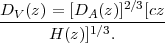
As with normal sound waves, one can usefully view the BAO phenomenon from different linear basis sets. We first consider the response to a density perturbation at a particular initial location, as illustrated in Figure 10; see Eisenstein et al. (2007b) and Eisenstein and Bennett (2008) for further description of this view. Primordial perturbations of the adiabatic form predicted by standard inflation models consist of equal fractional density contrasts in all species. The dark matter perturbation grows in place, slowly at first in the radiation dominated epoch, then faster as the universe becomes matter dominated. The baryon-photon perturbation, on the other hand, travels away from its origin as a sound wave. At recombination, the baryon part of the wave is left in a spherical shell centered on the original perturbation. Both the dark matter at the center and the baryons on the shell seed gravitational instability, which grows to form the halos in which galaxies form. We therefore expect the distribution of separations of pairs of galaxies (i.e., the two-point correlation function generated by such perturbations) to show a small enhancement at the radius of the shell, with galaxy concentrations in the central dark matter clumps and in the shells induced by the baryons.
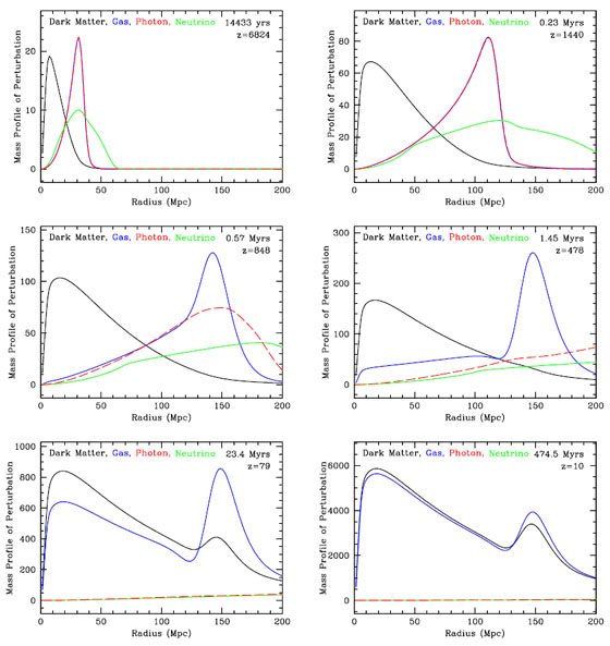 |
Figure 10. The generation of the acoustic peak illustrated via the linear-theory response to an initially point-like overdensity at the origin; this figure is reproduced from Eisenstein et al. (2007b). Each panel shows the radial perturbed mass profile in each of the four species: dark matter (black), baryons (blue), photons (red), and neutrinos (green). The redshift and time after the Big Bang are given in each panel. All perturbations are fractional for that species. We have multiplied the radial density profile of the perturbation by the square of the radius in order to yield the mass profile. In detail, we begin with a compact but smooth profile at the origin, which is why the mass profiles go to zero there. As we are using linear theory, the normalization of the amplitude of the perturbation (and thus the absolute scale of the y-axis) is arbitrary. a) Near the initial time, the photons and baryons are tightly coupled in a spherical traveling wave. b) The outward-going wave of baryons and relativistic species increases the perturbation of the cold dark matter, similar to raising a wake. c) At recombination, the photons decouple from the baryons. d) With recombination complete, the CDM perturbation is near the origin, while the baryonic perturbation is in a shell of 150 Mpc. e) With pressure forces now small, baryons and dark matter are attracted to these overdensities by gravitational instability. f) Because most of the growth is drawn from the homogeneous bulk, the baryon fraction converges toward the cosmic mean at late times. Galaxy formation is favored near the origin and at a radius of 150 Mpc. These figures were made by suitable transforms of the transfer functions created by CMBfast (Seljak and Zaldarriaga 1996, Zaldarriaga and Seljak 2000). |
One can equally well view the BAO effect as a standing wave in Fourier space; see Hu and Sugiyama (1996) and Eisenstein and Hu (1998) for this explanation. In Fourier space, the single acoustic scale gives rise to a harmonic sequence of oscillations in the power spectrum. This is easy to understand physically. The power spectrum encodes the response of the universe to a plane wave perturbation. Each crest in the initial wave produces a planar sound wave that travels a distance equal to the acoustic scale. If the wave deposits the baryon perturbation on another crest of the dark matter perturbation, then one gets constructive interference; if the sound wave ends in a dark matter trough, one gets destructive interference. The result is a harmonic relation between the wavelength of the perturbation and the acoustic scale.
Mathematically, this correspondence can be seen by considering that the correlation function and power spectrum are Fourier transform pairs. The Fourier transform of a delta function is a sinusoid, and the smearing of a delta function simply provides a damping envelope to that sinusoid. In the case of the BAO, this smearing is largely due to Silk damping in the early universe and to non-linear structure formation at late times. Both cause the higher harmonics in the power spectrum to be reduced in amplitude or washed out.
While it is secondary to our pedagogical thread, we end with some additional discussion of Figure 10 and the evolution of the initial point-like density perturbation. First, because the perturbation is in the growing mode, only the density perturbation is localized. The velocity perturbation away from the initial density perturbation has zero divergence but is non-zero; hence it scales as r-2 at large radius. As the baryon-photon and neutrino pulses expand, the gravity interior to the shell is weaker than it would have been. This causes the velocity perturbation interior to grow less quickly, creating a non-zero divergence away from the origin, which is why the CDM perturbation grows at non-zero radius. The size of this effect depends on the radiation to matter density; this transformation of the CDM perturbation is the famous k-2 tail of the CDM transfer function (Peebles 1982). The non-zero velocity perturbation is also the reason why the neutrino perturbation does not remain as a sharp peak. Finally, we note that this description of the behavior is the Green's function of the system. CMB Boltzmann codes typically compute the evolution of individual Fourier standing waves; these are simply combined here to generate the response to a point perturbation rather than a single standing wave.
4.3.2. Non-linear Evolution and Galaxy Clustering Bias
The clustering of matter and galaxies undergoes substantial changes at low redshift beyond the growth described by linear perturbation theory. Small-scale structure grows non-linearly, peculiar velocities behave differently from their linear prediction, and galaxies trace the dark matter in a complicated manner. We should worry that these effects might modify the location of the BAO feature relative to the prediction of linear theory, thus distorting our standard ruler (Meiksin et al. 1999, Seo and Eisenstein 2005, Angulo et al. 2005, Springel et al. 2005, Jeong and Komatsu 2006, Huff et al. 2007, Angulo et al. 2008, Wagner et al. 2008).
Fortunately, the large scale of the acoustic peak insulates it from most of non-linear structure formation (Eisenstein et al. 2007b). A typical pair of dark matter particles changes its comoving separation by 10 h-1 Mpc (rms value) between high redshift and z = 0. These motions broaden the acoustic peak, but the rms displacement is only mildly larger than the 8 h-1 Mpc scale set by Silk damping. The apparent displacement along the line of sight is larger in redshift space, because the peculiar velocity is well correlated with the displacement. Figure 11 shows the correlation function and power spectrum from N-body simulations; one can see that the acoustic peak in the correlation function becomes broader at low redshift. The corresponding effect in the power spectrum is the decreased amplitude of the wiggles at higher wavenumber. Roughly speaking, one can think of the width of the evolved ξ(r) peak as the quadrature sum of the initial width and the rms pairwise displacement Σnl (see Orban and Weinberg 2011, who examine idealized BAO models numerically and analytically). Equivalently, the oscillations in P(k) are damped by a factor exp(-k2Σnl2). As discussed in Section 4.3.4, the broadening of the BAO feature does not significantly bias the acoustic scale measurement provided one is using a suitable template-fitting method. However, it does degrade the precision of the measurement for a given survey volume, as it is harder to centroid a broader feature.
 |
Figure 11. The effects of non-linear clustering on the BAO. (Left) Redshift-space matter correlation function at four different redshifts from the simulations of Seo and Eisenstein (2005). (Right) Real-space matter power spectra at four different redshifts from the simulations of Seo et al. (2008), divided by a smooth power spectrum so as to reveal the acoustic oscillations. The input linear theory is shown by the dashed line. The effects of non-linear structure formation broaden the acoustic peak in the correlation function. In the power spectrum, this corresponds to a damping of the higher harmonics. Importantly, the boost of broad-band power at late times visible in the power spectrum plot corresponds largely to correlations at scales much smaller than the acoustic peak. |
To change the acoustic scale itself, one needs instead to move pairs systematically closer or systematically further away. This is a much weaker effect than the rms motion of particles, as it depends on the density variations in 150 Mpc spheres, which are percent level. Moreover, pairs of overdensities fall toward each other and pairs of underdensities fall away from each other, and both situations count equally toward a two-point statistic, causing a partial cancellation.
Padmanabhan and White (2009) compute the change in the acoustic peak location at second-order in gravitational perturbation theory. Crocce and Scoccimarro (2008) have done similar calculations in renormalized perturbation theory. Both calculations reveal a second-order term of the form dξ / dr, which corresponds to moving the acoustic peak. Padmanabhan and White (2009) compute the size of this effect to be around 0.25% at z = 0.
N-body simulations reveal a similar story. Seo et al. (2010b) measure the shift in the acoustic scale in a large volume of simulations and detect a shift from α = 1 of 0.3% ± 0.015% at z = 0.0, with a scaling in redshift proportional to the square of the linear growth function as expected for a second order effect (left panel of ). Padmanabhan and White (2009) validate their analytic calculation with a similar set of simulations.
Redshift-space distortions have further effects on the BAO signal beyond the extra broadening from the large-scale peculiar velocity. Small-scale velocities, e.g., the Finger of God effect, blurs the measurement of clustering along the line of sight, thereby broadening the acoustic peak. Moreover, the peculiar velocities create anisotropy in the broadband clustering, which must be carefully accounted for when extracting the acoustic scale (Section 4.3.4).
Linear bias, with galaxy density contrast δg = bδm, changes the amplitude of ξ(r) or P(k) but not the shape. However, any realistic bias relation must be at least somewhat non-linear, which alters the relative weighting of overdense and underdense regions and should shift the acoustic scale at second order. Early work attempted to measure this shift in simulations (Seo and Eisenstein 2003, Angulo et al. 2008), but the volume of the simulations was insufficient to get a conclusive detection of the effect. More recently, Padmanabhan and White (2009) explored galaxy bias as the ratio of the second-order to first-order bias term, finding shifts of a few tenths of a percent for reasonable bias cases. Mehta et al. (2011) treated the problem numerically with halo occupation distributions, finding shifts of 0.1% to 0.8% at z = 1 depending on the strength of the bias (right panel of figure 12). For halo-based models or other prescriptions that tie galaxy bias to the local density field, it therefore appears that bias-induced shifts are small, and corrections of modest fractional accuracy (e.g., to 20% of the shift itself) will suffice to make them negligible. The relevant bias parameters should be tightly constrained by smaller scale clustering measurements and higher order statistics, enabling cross-checks of the model used for correction.
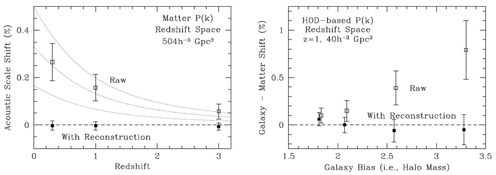 |
Figure 12. The shifts of the acoustic scale in cosmological N-body simulations. (Left) Shifts of the acoustic scale in the redshift-space matter power spectrum versus redshift from Seo et al. (2010b). The open symbols show the acoustic scale shifts prior to reconstruction; the dashed lines show a scaling of the square of the linear growth function. The solid symbols show the shifts after reconstruction is applied. The error bars are derived from the variance among simulations. (Right) Shifts of the acoustic scale in the redshift-space power spectrum of mock galaxy distributions at z = 1 from Mehta et al. (2011). The acoustic scale shift from the matter distribution in the same boxes has been subtracted so as to decrease sample variance. Galaxies are placed via HOD prescriptions; increasing mass thresholds leads to lower number densities and higher clustering bias. The open symbols show the shifts prior to reconstruction; the solid symbols, after reconstruction. The errors in the right panel are larger due to the smaller simulated volume and the lower number density of tracers. In all cases of both panels, reconstruction decreases the errors on the acoustic scale and reduces the shift to be consistent with zero. The left panel is based on 63 simulations, each using 5763 particles in a 2 h-1 Gpc cube. The right panel is based on 40 simulations, each with 10243 particles in a 1 h-1 Gpc cube. |
Non-local bias models that tie galaxy formation efficiency directly to the environment on much larger scales (e.g., Babul and White 1991, Bower et al. 1993) could perhaps induce larger shifts of the acoustic scale. However, such models require fairly extreme physical effects, and they can be readily diagnosed via their impact on clustering at scales below the BAO scale (Narayanan et al. 2000). A survey capable of measuring the acoustic scale to the sub-percent statistical level will provide in its millions of galaxies extensive opportunities to constrain even very general bias models accurately enough to predict the acoustic scale shift to within 10-20% of its value, sufficient to bring the systematic error below the statistical error.
By broadening and shifting the BAO feature in ξ(r), non-linear gravitational evolution degrades BAO precision and introduces a possible systematic. Is it possible to remove these effects by "running gravity backwards" to reconstruct the linear density field? The Zel'dovich (1970) approximation — in which particles follow straight line trajectories in comoving coordinates at the rate predicted by linear perturbation theory — captures important aspects of non-linear evolution on large scales (e.g., Weinberg and Gunn 1990, Melott et al. 1994). Eisenstein et al. (2007a) show that a simple reconstruction scheme based on applying the (reversed) Zel'dovich approximation to the smoothed non-linear density field is remarkably successful at recovering BAO information, effectively shifting the low redshift curves in Figure 11 back towards the high redshift curves. Figure 13, from Padmanabhan et al. (2012), illustrates how reconstruction works in the idealized case of an initial perturbation that exactly mimics the "acoustic ring" pattern.
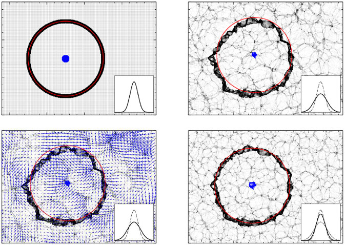 |
Figure 13. A pedagogical illustration of how reconstruction can improve the measurement of the acoustic scale; this figure is from Padmanabhan et al. (2012). Each panel shows a thin slice of a cosmological density field. (Top Left) At early times, the density is nearly constant. We mark a set of points at the origin in blue and a ring of points at 150 Mpc in heavy black. We measure the distances between the black points and the centroid of the blue point; the rms of these distances is represented by the Gaussian in the inset. (Top Right) At later times, structure has formed (in this calculation, simply by the Zel'dovich approximation), and the points have moved. The red circle shows the initial radius of the ring, centered on the current centroid of the blue points. The fact that the black points no longer fall on the red ring indicates that the acoustic peak has been broadened. The inset shows that the new rms of the radial distance (solid line) is larger than the original (dashed line). (Bottom Left) Arrows show the Zel'dovich displacements responsible for the structure that has formed. The idea of reconstruction is to estimate these displacements and move the particles back. (Bottom Right) We illustrate this by smoothing the density field by a 10h-1 Mpc filter and moving the particles back. Because the displacement field is imperfectly estimated, small-scale structure remains. But the black points now fall closer to the red ring, so that the rms of the radial distance is close to the initial (inset). The actual reconstruction algorithm of Padmanabhan et al. (2012) is more complex, but this example shows the basic opportunity. |
Seo and Eisenstein (2007) and Seo et al. (2010b) investigate the effects of reconstruction in more detail, showing that it noticeably improves the scatter and decreases the shift of the recovered acoustic scale from the matter density field of N-body simulations. The latest simulations demonstrate that the non-linear shift of the scale has been removed to 0.02% or better (see Figure 12, left). Moreover, comparing the initial conditions to final conditions on a mode-by-mode basis shows that the linear density field has been recovered to roughly double the pre-reconstruction wavenumber. Padmanabhan et al. (2009) analyze the method analytically, revealing the improvement while also noting that the recovered density field is not exactly the linear one.
Mehta et al. (2011) extend this analysis to HOD-based mock galaxy catalogs in simulations. They consider a range of HOD prescriptions and find that the reconstruction of the linear density field is not degraded by this form of galaxy bias and that the shift of the acoustic scale after reconstruction still vanishes, this time to 0.1% precision (Figure 12, right). This success is not surprising: the halo field traces the matter field fairly accurately on the scales required for reconstruction, so one is correctly estimating and removing the large scale displacements. Non-linear galaxy bias still alters the weighting of convergent and divergent flows, but if the flows are being mostly removed, then it doesn't matter how they are weighted.
Reconstruction is thus a powerful tool: one is achieving better statistical precision for a given survey, typically by a factor of 1.5 to 2, equivalent to a factor of 2-4 increase in survey size. Meanwhile, one is mitigating the primary systematic error from non-linear clustering and galaxy bias. As an added benefit, one can use the estimate of the large scale displacements to remove large-scale redshift-space distortions, 26 as illustrated in Figure 14, which decreases that degradation of the BAO accuracy and also pushes most of the BAO signal into the monopole and quadrupole components of ξ(s) or P(k). Without reconstruction, the redshift-space distortions contain significant terms in the hexadecapole and beyond, and the quadrupolar squashing of the Alcock-Paczynski effect couples to the quadrupole redshift-space distortion to produce BAO signal in the hexadecapole. To the extent that one is recovering the linear density field, one can also hope that the large-scale density field is more Gaussian, which is a major simplification for computing likelihood functions. However, this last property has not been extensively tested.
 |
Figure 14. The ability of reconstruction to correct redshift-space distortion of the BAO feature; figure panels taken from Padmanabhan et al. (2012). The left panel shows contours of the galaxy correlation function from N-body mock catalogs, multiplied by r2 to enhance the large scale features, as a function of transverse (r⊥) and line-of-sight (r∥) separation. Apart from statistical fluctuations, this correlation function is isotropic. The middle panel shows contours of the galaxy correlation function in redshift-space. Peculiar velocities induce anisotropy, breaking the BAO ring into two arcs. The right panel shows the redshift-space correlation function of the galaxy distribution after reconstruction, including peculiar velocity correction at the level of the Zel'dovich approximation, which largely restores the isotropy of the BAO ring. |
The first applications of BAO reconstruction to observational data appear in Padmanabhan et al. (2012) and Anderson et al. (2012). For the SDSS-II (DR7) LRG sample, reconstruction shrinks the BAO distance error from 3.5% to 1.9%, equivalent to a factor of three increase in survey volume. It also improves the agreement between the observed and predicted shapes of the correlation function in the BAO regime, thereby increasing the statistical significance of the BAO detection from 3.3σ to 4.2σ. For the BOSS (DR9) sample, reconstruction produces little improvement in the BAO measurement, although this is consistent with the variation among DR9 mock catalogs (see discussion by Anderson et al. 2012).
There is an extensive literature on reconstruction methods for large-scale structure (e.g., Peebles 1989, Weinberg 1992, Nusser and Dekel 1992, Croft and Gaztanaga 1997, Narayanan and Weinberg 1998, Mohayaee et al. 2006). Even simple methods appear adequate for BAO recovery, but better reconstruction is valuable for other applications of large-scale structure (Reid et al. 2010). Since BAO surveys are typically sparse, an important area for continuing research is the performance of methods in the presence of both galaxy bias and significant shot noise. The effectiveness of reconstruction as a function of sampling density might have important implications for survey design, favoring different choices compared to the statistical considerations discussed in Section 4.4 below.
It is worth stressing that "the acoustic scale" is only an approximate description of a more complicated physical situation. For high precision work, we cannot separate the concept of the acoustic scale from the context of a Boltzmann code prediction for the matter power spectrum and CMB anisotropy power spectrum. The sound horizon defined by equation (52) does not correspond to the exact maximum of the acoustic peak in the correlation function, nor do the harmonics in the matter power spectrum have an identical scale to those in the CMB anisotropy spectrum. The differences arise from effects such as the fact that photons decouple from the baryons earlier than the baryons decouple from the photons, that the post-recombination matter growing mode is largely set by the velocity perturbation at recombination rather than the density perturbation, and that Silk damping alters the effective redshift of recombination as a function of wavenumber. These effects are accurately calculated in the Boltzmann codes, resulting in precise predictions for the matter and CMB power spectra.
When one wants to extract the acoustic scale (i.e., to measure distance using the BAO standard ruler) from a measurement of the two-point clustering, the appropriate thing to do is to use the predicted clustering for the cosmology one is testing as a template. The optimal plan is then to fit that template to the data over a range of scales using the correct covariance matrix or likelihood. Some early works instead used non-parametric models for the acoustic peak, such as a Gaussian in configuration space or a damped sinusoid in Fourier space (Blake and Glazebrook 2003), or simply identified the maximum of the correlation function (Guzik et al. 2007, Smith et al. 2008). We believe that, because the acoustic scale is predicted only in the context of an early universe model with parameters taken from fits to CMB data, there is no extra value in avoiding the linear-theory model predictions.
Having said that, one does want to modify the template to allow for effects of non-linear structure formation and perhaps to marginalize over broad-band terms that might enter from scale-dependent clustering bias or velocity bias or from errors in the calibration of one's survey. This procedure has been carried out by several different authors. For example, Seo and Eisenstein (2007) and and Seo et al. (2010b) fit the measured power spectrum to the form
 |
(54) |
where A(k) and B(k) are smooth functions with parameters to be fit. Pm(k) is the linear theory model with the acoustic oscillations additionally damped by large-scale structure,
 |
(55) |
where Σnl is a constant fit from simulations. Pnw is the no-wiggle power spectrum from Eisenstein and Hu (1998), hand-crafted to edit out the acoustic oscillations. Plin is the exact linear theory power spectrum; note that Pm(k) goes to this exact linear theory result in the limit of negligible damping (Σnl → 0), so the approximate form of Pnw(k) is acceptable. The broadband terms A(k) and B(k) will correct for non-linear power, the shot noise, scale-dependent bias, and any imperfections in the survey. The primary goal for the fit is to measure α, a factor that dilates the scale of the predicted clustering (and of the BAO feature in particular) relative to the observed clustering. A value α=1 indicates agreement with the acoustic scale of the original model. A value α1 indicates that the acoustic scale of the linear-theory model is incorrect or that the distance scale assumed in measuring the galaxy clustering was wrong. Simple alterations of this prescription can be made for fitting the correlation function or mixed-space ω or wavelet statistics (Xu et al. 2010, Arnalte-Mur et al. 2012). This appproach thus allows one to fit for the scale of a standard ruler without having to recompute a full predicted power spectrum at every point in parameter space.
This fitting procedure is only compelling to the extent that the recovered value of α is stable (to within the statistical errors) as one varies the prescription for the marginalization of parameters in A(k) and B(k). Too little freedom and one may be biased by broadband tilts and modulations that one hasn't modelled properly; too much freedom and one will fit out the acoustic signature and reduce the constraining power of the data. Fortunately, the separation between the acoustic scale and the typical non-linear scale and Silk damping scale is large, i.e., the acoustic peak in the correlation function is narrow. This gives considerable freedom to fit away broadband nuisance terms while not impacting the acoustic peak. Seo et al. (2010b) show stable results for α for various choices, e.g., polynomials of different order. Similarly, α is robust to changes in the choice of Σnl, so one is not sensitive to how one estimates that parameter in simulations or mock catalogs.
An equivalent method has been used by Percival et al. (2007), Percival et al. (2010), and in related works. Here, one fits a spline to the measured power spectrum and divides by that spline. One does similarly for the template Pm(k) and fits that to the residual spectrum of the data. This is equivalent to taking B(k) to be a spline and setting A(k) = 0. Clearly the performance depends on the number of spline points, but there is a broad stable region.
The definition of the acoustic scale as the distance a primordial sound wave could travel before recombination (eq. 52) is borne out in such fits. If one fits with the power spectrum from a cosmology that is moderately wrong, then one infers a different α, but this change in α is proportional to the ratio of the acoustic scales, as defined by the sound horizon integral for each cosmology. The stability of this scaling appears to be much better than the statistical errors implied by the surveys that are defining the range of interesting cosmological parameter space (Seo et al. 2010b). In other words, one can use the acoustic scale integral to adjust distance scale measurements of DA / rs and Hrs between different cosmologies within the domain of interest.
Extending these approaches to the anisotropic case so as to extract DA and H separately is more complicated and has not been fully developed. The primary obstacle is to account for the anisotropic distortions from peculiar velocities. Examples of fit methodologies include Okumura et al. (2008), Padmanabhan and White (2009), Shoji et al. (2009), Chuang and Wang (2012), Kazin et al. (2012), and Xu et al. (2012a). The ability of reconstruction to mitigate peculiar velocity distortion (Fig. 14) may be a significant asset for disentangling DA and H.
With better modeling of non-linear structure and galaxy clustering bias, one could of course extract additional cosmological information from the two-point clustering of galaxies. In particular, one can measure the distance scale from the curvature (i.e., non-power-law form) of the spherically-averaged power spectrum or correlation function. This physical scale arises from the size of the horizon at matter-radiation equality, parameterized as Ωm h2 in typical cosmologies. However, this curvature is a much broader feature and thus provides less leverage on distance. Most important, the width of the feature is comparable to the scale itself, implying that one must control all extra broad-band sources of power and scale-dependent galaxy biases in order to extract accurate distance information. This is much more challenging than the BAO application, but it is an important frontier of the field of large-scale structure. In particular, the application of this approach to the quadrupole distortion known as the Alcock-Paczynski effect will be discussed in Section 7.3.
4.4. Observational Considerations
The primary challenge of the BAO method is that very large samples of galaxies (or other tracers) are required to detect the acoustic oscillations and hence measure a distance. Like detecting an emission line in a galaxy spectrum in order to measure a redshift, one must have high enough signal-to-noise to detect the BAO peak or one gets no useful distance information at all. The minimum useful survey volumes are of order 1h-3 Gpc3, which yield a distance precision of about 5%.
The two components of the statistical error are sample variance and shot noise (Kaiser 1986a). A given survey volume contains only a certain number of Fourier modes; in the periodic box approximation dNmodes / dk = 4π k2 V / [(2π)32], where the final factor of 2 in the denominator accounts for the fact that the density field is real. In a Gaussian random field, the real and imaginary parts of each mode are independent with an intrinsic variance of P(k)/2. In addition, each mode is imperfectly measured due to shot noise; when treated in the Gaussian approximation (ignoring the 4-point contributions from the Poisson distribution), this raises the variance on the square of the complex norm to [P(k) + 1 / n]2, where n is the number density of tracers. The result is that the fractional error bar on the measurement of each mode is σp / P = (nP + 1) / nP. When combining information from modes, we should sum the inverse variances, which are
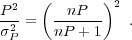 |
(56) |
We see that for n ≫ 1 / P(k) we get unit information from each mode but that the information drops rapidly for n < 1 / P(k). We note that the relevant P is the redshift-space power spectrum; this can be substantially larger than the real-space power spectrum for nearly radial large-scale modes, thereby decreasing the shot noise impact on BAO estimation of the Hubble parameter.
The mode-counting argument above neglects boundary effects, effectively assuming that the survey volume is reasonably contiguous with a high filling factor on scales of 150 Mpc. In real space, we can express this as the requirement that the number of pairs of survey galaxies at 150 Mpc separation not be significantly diminished compared to the case of a filled periodic box. In Fourier space, we must ensure that the survey window function not create aliasing between modes in the crests and troughs of the acoustic oscillations.
Converting a power spectrum forecast into constraints on the distance scale requires marginalizing over other cosmological parameters. This has been done with Fisher matrix analyses (Seo and Eisenstein 2003, Seo and Eisenstein 2007) or with Monte Carlo approaches (Blake and Glazebrook 2003, Glazebrook and Blake 2005, Blake et al. 2006). Several analyses have focused on the anisotropy of the power spectrum in order to measure H(z) and DA(z) separately.
Seo and Eisenstein (2007) constructed a fast approximation to the full Fisher matrix calculation using an idealized treatment of the acoustic oscillation, including non-linear structure formation and redshift-space distortions. This method allows forecasts for H and DA precision as a function of survey redshift, number density, and volume (see their eq. 26). Tests with simulations (Seo et al. 2010b, Mehta et al. 2011) have shown this forecast to be accurate to within 10-20%, with a small trend toward over-optimism at nP < 1. Whether this trend is intrinsic to shot noise or to the fact that the low number density models used more massive mass thresholds for halo bias is not clear at present.
Table 2 presents a summary of cosmic variance limited BAO performance. This is a tabulation of the Seo and Eisenstein (2007) forecasts for a full-sky survey, using even binning in ln(1 + z). We assume a shot noise level of nP = 2 at k = 0.2 h Mpc-1 (see Section 4.4.3), and that reconstruction has decreased the non-linear displacements by a factor of two in length scale, i.e., reducing the quantity Σnl in equation (55) by a factor of two below its full non-linear value at each redshift. Figure 15, discussed further in the next section, presents graphical summaries of the main features of Table 2. One can see that the precision available in DA(z) and H(z) is excellent: of order 0.2% per redshift bin at high redshift. At low redshift, the precision is worse because there is far less cosmic volume. Of course, these statistical errors scale as fsky-1/2, where fsky is the fraction of sky surveyed.
| zmin | zmax | Volume | % Err DA(z) | % Err H(z) | ΩΛ(z) | S/N | σw |
| 0.00 | 0.15 | 0.33 | 2.8 | 4.9 | 0.708 | 7.3 | 0.64 |
| 0.15 | 0.32 | 2.62 | 0.95 | 1.7 | 0.616 | 18.2 | 0.088 |
| 0.32 | 0.51 | 7.89 | 0.53 | 0.96 | 0.515 | 27.0 | 0.036 |
| 0.51 | 0.73 | 16.5 | 0.35 | 0.63 | 0.413 | 32.9 | 0.021 |
| 0.73 | 0.99 | 28.4 | 0.26 | 0.46 | 0.318 | 34.9 | 0.015 |
| 0.99 | 1.28 | 42.9 | 0.21 | 0.36 | 0.236 | 33.3 | 0.013 |
| 1.28 | 1.62 | 59.0 | 0.17 | 0.28 | 0.170 | 30.2 | 0.012 |
| 1.62 | 2.00 | 75.8 | 0.14 | 0.24 | 0.119 | 25.2 | 0.013 |
| 2.00 | 2.44 | 92.3 | 0.13 | 0.21 | 0.082 | 20.0 | 0.014 |
| 2.44 | 2.95 | 108 | 0.12 | 0.18 | 0.056 | 15.5 | 0.016 |
| 2.95 | 3.53 | 121 | 0.11 | 0.17 | 0.038 | 11.4 | 0.020 |
| 3.53 | 4.20 | 133 | 0.10 | 0.15 | 0.025 | 8.3 | 0.025 |
| 4.20 | 4.96 | 142 | 0.10 | 0.15 | 0.017 | 5.8 | 0.033 |
| These forecasts assume a full-sky survey, use nP = 2 at k = 0.2 h Mpc-1, and assume reconstruction improvements in the non-linear damping by a factor of 2. Statistical errors scale as fsky-1/2. The first and second columns give the inner and outer edges of redshift bins; the bins have equal width in ln(1 + z). The third column gives the comoving volume of the bin in h-3 Gpc3, assuming Ωm = 0.25. The fourth and fifth columns give 1σ fractional errors (in percent) in DA(z) and H(z), the angular diameter distance to and Hubble parameter at the bin center; note that the errors on these two quantities are 40% correlated. We assume the sound horizon is known. The sixth column gives ΩΛ(z), i.e., the ratio of the dark energy density to the critical density at that redshift in a Λ-model. Column 7 gives ΩΛ(z) H / 2σh, which is the significance at which one would detect the cosmological constant at redshift z using only the H(z) BAO constraint and assuming perfect knowledge of the matter density and curvature (a good approximation, but not exact). Column 8 shows the error on a constant value of w that would be obtained by comparing the BAO H(z) measurement for this one redshift to the value of ρDE at z = 0, assuming the latter is known perfectly. | |||||||
4.4.2. From BAO to Dark Energy
We will explore how these performance estimates map to dark energy parameter forecasts in Section 8, but here we describe some simplified treatments in order to build intuition. Beginning at low redshift, if we consider that CMB anisotropies give precise values for Ωm h2 and the acoustic scale rs, then a BAO detection near z = 0 is measuring a standard ruler and hence H0 (Eisenstein and Hu 1998). Combining that with Ωm h2 yields Ωm. No BAO measurement can be strictly at z = 0, but the inference of Ωm and H0 depends only on the distance scale between z = 0 and the survey redshift. Even at z = 0.35, this brings in only a mild dependence on w and Ωk (Eisenstein et al. 2005). Hence, low-redshift BAO measurements offer a strong measurement of Ωm. Determining Ωm breaks a key degeneracy for the SN measurements between Ωm and w.
Moving to higher redshift (z ≳ 1), we next consider the evolution of the density of dark energy using only the H(z) information from BAO (right panel of Figure 15). If we know the matter density and spatial curvature perfectly, then the Friedmann equation directly relates the measurement of H(z) to the density of dark energy at that redshift. Considering the null hypothesis of the cosmological constant, we would achieve a detection of the dark energy density with a significance of ΩΛ H / 2σ(H), where σ(H) is the error on H(z). We next want to consider the variation in the dark energy density. Taking an example in which one assumes the z = 0 value is known perfectly, we can translate the error at a given redshift to the error on the exponent of a power-law variation, which can in turn be rewritten as an error on a constant w (eq. 23). Of course, a full analysis must include the uncertainties on the matter density, spatial curvature, and z = 0 value of ΩΛ.
 |
Figure 15. Illustrative BAO forecasts for a full-sky survey, from Table 2. All errors scale as fsky-1/2; note that y-axes are inverted so that smaller errors appear higher on the plot. (Left) The fractional error on DA(z) and H(z) in logarithmic redshift bins, as open and solid points, respectively. Note that performance of order 0.2% per bin is possible at high redshift. Here we assume the sound horizon is known. (Right) Illustration of the dark energy leverage available simply from the H(z) information in the previous panel. Assuming perfect knowledge of the matter density (i.e., Ωm H02) and curvature, measurement of H(z) determines the dark energy density. The solid black points show the resulting fractional errors on the dark energy density as a function of redshift, assuming that the value is close to the cosmological constant. Errors of order 5%, i.e., a 20-σ detection of dark energy, are possible at 0.5 < z < 2, even if the dark energy density is simply constant. The evolution of dark energy can be expressed by comparing the density at high redshift to that at z = 0, assuming the latter is known. The open red points give the error on a power-law evolution in 1 + z, expressed as the error on a constant w. One sees that there is a broad maximum in performance extending out to z ≈ 3. Of course, we must measure the dark energy density at z = 0; the blue arrow shows the fractional error on that density that would result from a 1% measurement of H0 (which one might get from direct measures or from a combination of BAO and supernovae), assuming perfect knowledge of the matter density. That the blue arrow is comparable to or above the solid points indicates that we can reasonably expect to be limited by our higher redshift data. The open points are optimistic in that we have assumed perfect knowledge of various inputs; the intended lesson is that the large volume and larger redshift lever arm at higher redshift can offset the fact that the dark energy makes up a smaller fraction of the cosmic total. |
Despite the simplifications, Table 2 and Figure 15 offer some important results for building intuition. We find that the sensitivity of BAO H(z) to dark energy has a broad maximum over the range 0.6 < z < 3.5. This plateau arises because the declining dynamical importance of dark energy is compensated by the increasing statistical precision afforded by larger comoving volume. For w=-1, dark energy is only 10% of the total density at z = 2, but a cosmic-variance-limited BAO measurement can detect that density at 20-σ significance. The large lever arm to z = 0 translates this into a 1.3% constraint on a constant w model. Of course, if w > -1, then ρDE is higher at high redshift than it is for a cosmological constant, increasing the statistical significance with which BAO can detect it.
Meanwhile, the transverse acoustic scale at z~2 and above can be compared to the angular acoustic scale in the CMB to give a combination constraint on early dark energy and the curvature of the universe (McDonald and Eisenstein 2007). This has considerable value in breaking degeneracies between curvature and dark energy parameters at lower redshift, and it should be considered an important consistency check for the ΛCDM interpretation of the CMB. A clear detection of non-zero curvature would have major implications for inflation, and perhaps for quantum cosmology theories (Gott 1982, Guth and Nomura 2012, Kleban and Schillo 2012). If the Alcock-Paczynski method can be applied at smaller scales to obtain a precise determination of H(z) DA(z), then the BAO values of DA(z) can also be used to improve H(z) determinations and thus the dark energy density constraints (see Section 7.3).
The acoustic oscillations in the power spectrum are primarily at wavenumbers 0.1-0.2 h Mpc-1, so we want to design surveys with nP(k = 0.2 h Mpc-1) ≳ 1. Furthermore, if one wins sample size proportionally to survey time, then nP(k) = 1 is the optimal balance of survey depth to sample volume at a given wavenumber (Kaiser 1986a). One should beware that this assumption rarely holds in surveys with multi-object instruments: the exposure time is driven by the faintest objects in the survey, so that brighter galaxies are being overexposed in the chosen observation time. Also, the number density is often a function of redshift, so one cannot hit the optimal density everywhere in the survey. Finally, one might care about distance precision differently at different redshifts because of one's specific goals for testing dark energy models. See Parkinson et al. (2007) for a worked example of survey optimization.
For the concordance cosmology, the amplitude of the power spectrum at k = 0.2 h Mpc-1 is about 2700σ8,g2 h-3 Mpc3, where σ8,g2 is the variance of the fractional overdensity of the chosen tracer at the survey redshift in spheres of 8h-1 Mpc radius. This implies that we seek number densities around n = (4 × 10⁻⁴ h3 Mpc-3) / σ8,g2. Fortunately, this is well below the density of L* galaxies.
Higher galaxy bias is a good thing for the statistical errors of a BAO survey. The power spectrum amplitude scales as the square of the bias, so an early-type galaxy is 3-4 times more valuable (in the sense of boosting nP) than a late-type galaxy. Given that there is no identified risk — higher bias galaxies have larger acoustic scale shifts, but this is correctable (Figure 12, right) — it makes sense to use higher bias tracers when possible. However, lower bias tracers can be more effective if one can acquire their redshifts sufficiently quickly!
The balance of shot noise to sample variance is more complex in the case of surveys with the Lyα forest or HI intensity mapping. However, the idea is the same: one wants to make a map in which the pixel noise is dominated by sample variance, but not by much. The power at k = 0.2 h Mpc-1 corresponds roughly to density variance of 8 h-1 Mpc spheres. Hence, we seek to measure the density of individual regions of this size to a precision slightly better than the intrinsic rms for such volumes for the chosen tracer (i.e., bσ8). If one is measuring too well, one would prefer to do shallower measurements over a wider region. In the case of the Lyα forest, this criterion concerns both the areal density of the quasar sightlines and the signal-to-noise ratio of the spectra (McDonald and Eisenstein 2007, McQuinn and White 2011).
4.4.4. Spectroscopic vs. Photometric Redshifts
Photometric redshifts offer a cheap way to measure many galaxy redshifts and hence to measure the BAO (Seo and Eisenstein 2003, Glazebrook and Blake 2005, Dolney et al. 2006, Seo and Eisenstein 2007). However, the larger errors are a challenge. For velocity errors larger than 1000 km s-1 one is smearing out the acoustic scale along the line of sight and failing to measure H(z). Note that this scale is set by the width of the acoustic peak, not by the acoustic scale. One only retains full information with rms precision below 300 km s-1.
To measure DA(z), in principle precisions of σz/(1 + z) of 4% are enough. Worse precision causes catastrophic degradation because the oscillations in angular power at the front and back of the photometric redshift slab fall out of phase. Redshift precision of 3-4% yields poor constraints on the BAO per unit volume, with a rule of thumb that one needs ten times more volume for a photometric redshift survey than a spectroscopic survey (Blake and Bridle 2005, Seo and Eisenstein 2007). Better redshift precision reduces this gap. At z < 0.7, current and ongoing spectroscopic surveys are already covering 1/4 of the sky, so photometric redshift surveys are only competitive at higher redshifts. Extracting large-scale structure and BAO from photometric redshift surveys requires very stringent calibration and more extensive modeling than for spectroscopic surveys. Photometric surveys with many narrow bands offer an intermediate approach between imaging and spectroscopy, which may be advantageous in some regimes (Benmtez et al. 2009).
As we have seen, BAO surveys require surveys of very large volumes with modest sampling density. One wants to map a wide range of redshift so as to measure the history of expansion. The current generation of surveys are mapping of order 1 million galaxies, and approaching the cosmic variance limit at z > 1 requires of order 108 galaxies.
We have a lot of freedom in selecting the objects to trace the density field. Usually, we require isotropy of the selection but do not require that the selection be unchanging as a function of redshift. One is seeking to minimize the observational cost for a given well-sampled survey volume. There are many competing considerations (Glazebrook and Blake 2005). One desires a tracer with a strong spectroscopic signature to allow a redshift determination to about 300 km s-1 rms as fast as possible, with few catastrophic redshift errors. One desires a combination of density and clustering bias so that nP(k = 0.2h Mpc-1) ≳ 1. One desires a higher clustering bias, so that the required number density is lower; this allows one to use brighter objects and reduce exposure time. For targeted surveys, one desires that the tracer can be readily selected, so that one doesn't waste resources on undesired objects. In more detail, one desires photometric redshifts good enough that one can shape the n(z) profile in a way that keeps nP close to unity at high redshift without being swamped by low luminosity objects at low redshift. And, of course, the observed wavelength of the spectroscopic feature determines a great deal about the instrumentation.
Luminous red galaxies are an effective choice at lower redshifts. They have strong absorption features, notably the 4000E break, and high surface brightnesses to allow rapid spectroscopy. They have a high bias (b ~ 2) to reduce the required number density and hence the number of spectroscopic fibers. They are also easy to select with photometric redshifts: essentially they are the reddest galaxies at a given observed flux (Eisenstein et al. 2001).
As we work to z = 1 and beyond, the advantages of using emission-line galaxies increase. Red galaxies are very faint in the optical at z ≳ 1 because of K corrections, and the 4000E break moves into the infrared where the forest of OH sky glow lines makes spectroscopy more difficult. But the star formation rates of normal galaxies at z > 1 are about ten times higher than today, and this high star formation produces strong emission lines. These emission lines can be detected even when the stellar continuum cannot, and the galaxies with the strongest lines can be measured in remarkably little time. Spectral resolution of a few thousand is desirable to work between the OH sky glow lines and to resolve the [OII] doublet. The challenge is primarily one of selection, how to use photometric data to pick out the star forming galaxies with the strongest lines. Between the lower clustering bias and the failure rate on weaker-lined systems, one needs to survey many more blue galaxies than red. Current expectations are that the transition point from preferring red galaxies versus blue is z ≈ 1 (Glazebrook and Blake 2005 ). Slitless spectroscopy offers an alternative route to surveying emission line galaxies, without prior target selection (see Section 4.6).
Clusters of galaxies have been proposed as tracers (Angulo et al. 2005, Hütsi 2006). These can be readily found from imaging data sets but have the disadvantage that their nP does not reach unity. Also, acquiring spectroscopic redshifts for the clusters imposes requirements similar in area and depth to a red galaxy survey, so the gain in a highly multiplexed fiber survey is much smaller than one would expect based on numbers alone. Quasars have a similar problem of having nP < 1, but they are extremely luminous and easy to select. This makes them a possible target for a sparse, wide-field survey at z > 1 (Sawangwit et al. 2012), and they are readily added to a multi-fiber survey targeting emission line galaxies or LRGs at other redshifts.
Using the Lyα forest as a tracer is attractive because each spectrum yields many density measurements (effectively about 50) rather than just a single point in a map (White 2003, McDonald and Eisenstein 2007, Norman et al. 2009, McQuinn and White 2011). One wants to sample the width of the acoustic peak, which is about 20h-1 Mpc FWHM. This implies that one needs spectral resolution of only a few hundred and moderate angular density of the lines of sight, preferably about 100 per square degree. Quasars of this surface density are much brighter than the Lyman-break galaxies that would be required to match the effective sampling density. As one has little gain from reducing the photon noise errors to below the intrinsic variation of the forest on 10 h-1 Mpc scales, one can afford to use low signal-to-noise ratio spectra. The challenge here is systematics, as one must control the continuum of the quasar and the spectrophotometry of the measurements to utilize the spectral information. It is also possible that theory systematics associated with the state of the IGM enter; so far, IGM uncertainties have not been shown to affect BAO measurements from the forest, but the case has not been investigated as thoroughly as it has for galaxies. The recent detection of BAO in the Lyα forest at a scale and amplitude compatible with theoretical expectations (Busca et al. 2012, Slosar et al. 2013) is already encouraging, but much work remains to demonstrate that systematic effects are below the achievable level of statistical precision.
Star-forming galaxies also can be observed in the radio using the 21 cm line of neutral hydrogen. This is a much weaker line, but future generations of radio interferometers such as the Square Kilometer Array offer phenomenal survey speed because one can synthesize millions of simultaneous beams computationally. Such instruments could in principle achieve spectroscopic samples of 109 galaxies out to z = 2-3 (Abdalla and Rawlings 2005).
A different concept is that of 21 cm intensity mapping (Peterson et al. 2006, Ansari et al. 2008, Chang et al. 2008, Loeb and Wyithe 2008, Wyithe et al. 2008, Seo et al. 2010a). Here one does not identify individual galaxies but instead measures the combined emission of the 21 cm line from all galaxies in a volume of order 10 Mpc on a side. The fluctuations in the map encode the large-scale density field and hence the BAO. Relative to an interferometer like the SKA, one uses shorter baselines (around 300 meters) and a nearly filled aperture to maintain surface brightness sensitivity. 27 Because one is not resolving individual galaxies above the instrumental noise, one is using all of the neutral hydrogen even from low-mass galaxies. In principle, one can map the BAO to the cosmic variance limit out to z≈3 with new interferometric arrays. The challenge is foreground subtraction, as the cosmic signal is several orders of magnitude below the Galactic and extragalactic emission levels. A first detection of large-scale structure in redshifted 21 cm has been reported by Chang et al. (2010) by cross-correlating with an optical galaxy redshift survey at z = 0.8; cross-correlation removes foregrounds that are not themselves correlated with the optical galaxies. For intensity mapping to work on its own, one of course needs to measure the auto-correlation signal.
Unlike for the case of galaxies, diffuse HI mapping does not provide the mean level of emission (interferometers are not sensitive to this, and even if they were the Galactic emission would swamp extragalactic HI); therefore δHI is measured only up to a multiplicative constant. This does not present a problem for the BAO technique because one is using the shape and not the amplitude of the power spectrum. It does have an impact on redshift-space distortions (Section 7.2), as without the mean level one cannot turn the observable β into an estimate of the rate of growth of structure f σ8(z). This drawback is, however, also an opportunity to learn about astrophysics: measurement of βHI combined with independent knowledge of f σ8(z) would allow us to infer the mean HI signal and thus obtain the cosmic abundance of neutral gas as a function of time (Wyithe and Brown 2010).
4.5. Systematic Uncertainties and Strategies for Amelioration
Given that we seek to measure the acoustic scale and hence cosmic distance scale to a high level of precision, it is important to consider the systematic errors that could cause the inferred DA(z) / rs and H(z) rs to be incorrect. We consider three classes of systematic errors: (1) observational errors, in which one mis-measures the large-scale structure of the universe; (2) astrophysical errors, in which our model of large-scale structure for a given cosmology is incorrect; and (3) cosmological errors, in which we mispredict the sound horizon given our measurements because of new cosmological physics, either in the early universe or at late times.
4.5.1. Measurement Systematics
The measurement of large-scale structure requires the ability to produce a well-calibrated density map of the universe. The data need not be homogeneous in quality so long as the inhomogeneities are known well enough that one can correct for them statistically.
Observational errors involve imperfections in one's map of the density field. Examples of sources can be photometric miscalibrations of the input catalog, mis-assessments of the incompleteness in the input catalog, redshift failures or errors, incorrect tracking of the target selection, failure to correct for deleterious interactions between targets (e.g., fiber collisions), or imperfect assessment of the redshift distribution of the map. Another class of problems involves understanding of the errors of the map, as one must assess both the statistical properties of the density field and the point sampling of it by galaxies.
Fortunately, these issues have been extensively studied in the general context of the measurement of large-scale structure (e.g., Tegmark et al. 1998). BAO measurement itself is only a particular application of large-scale structure data, and it turns out to be a relatively easy one because the acoustic peak is narrow in scale and hence one has another differential opportunity in the experimental design. That is, one can compare the behavior at 150 Mpc separation to the average of that at 120 and 180 Mpc, so as to remove smooth errors. The only way to produce a non-smooth error is to have a sharply preferred scale in the systematic error.
For galaxy redshift surveys, there is wide expertise in how to calibrate surveys and track their selection functions, and there are many tests that can be employed to look for specific problems. Failing that, residual errors are often intrinsically radial or angular in their nature, so one can reject the purely radial and purely angular modes from a survey (Vogeley and Szalay 1996, Tegmark et al. 1998). This is a small cost in information content for an intrinsically 3-d field. A more targeted version of this idea is to use angular templates to remove systematic errors with particular angular dependence, e.g., survey depth variations due to sky brightness, seeing, or stellar density (Ho et al. 2008, Ross et al. 2011, Ross et al. 2012). A further related idea is that for a sharp scale in a systematic error to be a real threat, it must be sharp for three dimensional spheres of separation. For example, even if a survey has an error that is modulated on a circular field of view, the diameter of the field affects a range of 3-d separations at a given redshift simply because of the random orientations of pairs to the line-of-sight.
The BAO method is ultimately tied to the separation of galaxies, which depend on astrometric positions and redshifts. These quantities can be exquisitely well measured, and achieving 0.1% precision on one's astrometric and wavelength scale is easy. The concern about systematic errors in the map is that an erroneous tilt in the correlation function would cause one to mismeasure the centroid of the acoustic peak. This is a weaker effect, and one can marginalize against such tilts if one wants, using the techniques in Section 4.3.4.
In short, it is very likely that a reasonable design for a galaxy redshift survey will lead to sufficient accuracy for the BAO method. The greater challenge for such surveys is to control the clustering analysis for the broadband cosmological signals, which require a factor of more than ten better accuracy.
On the other hand, the observational systematics for the Lyα forest and 21 cm intensity mapping techniques are a serious concern. Here we are trying to use every spectral pixel for our mapping data, rather than differencing spectral pixels to measure a single redshift per object. Imperfections in the calibration of the spectra or the subtraction of sky emission or Galactic foregrounds will appear as cosmic structure.
For the Lyα forest, we measure the absorption by assuming that the quasar continuum is intrinsically smooth. However, even an unabsorbed spectrum would have variations due to the intrinsic spectrum of the quasar and any errors in the removal of the sky emissions or flat-fielding of the detector. We do not know the detailed unabsorbed quasar spectrum but instead need to estimate it from the ensemble properties of quasars or from fitting to less absorbed pixels. The BAO signal is a very weak modulation on large scales. Modeling errors far too weak to show up in any one spectrum could inject correlations that bias the BAO scale or simply increase the noise far above the expected sample variance. The most detailed discussions of systematic errors in large-scale Lyα forest measurements are those of McDonald et al. (2006) and Slosar et al. (2011). Measuring the scale of the BAO feature again appears much easier than determining the broad-band shape or absolute amplitude of the power spectrum. Studies to date have not identified observational problems that would prevent high precision BAO measurements, but the field is in its early days.
For 21 cm intensity mapping, we are looking for the correlations of the extragalactic line emission as a function of wavelength (redshift) and sky position. However, the Milky Way is producing synchrotron and free-free emission that is three orders of magnitude higher than the extragalactic signal and highly variable on the sky (2008Chang et al. , 2010Chang et al. ). Fortunately these emission mechanisms are smooth as a function of frequency, unlike the cosmological signal where frequency maps to redshift, which should enable foreground removal (e.g., Liu and Tegmark 2012). The challenge here is primarily instrumental: undesired features in radio interferometers such as far sidelobes or standing waves in the antenna are strongly frequency dependent and can mimic a cosmological signal if not suppressed. Moreover, the Galactic synchrotron radiation is polarized, and Faraday rotation within the galaxy can lead to strongly wavelength-dependent polarization amplitude (e.g., Haverkorn et al. 2003), so the instrument and software must measure the total intensity and remove Stokes Q and U from their maps — a major challenge given that radio antennas are inherently polarized. The problems are similar to those of the 21 cm mapping of the epoch of reionization, where several experiments are trying to achieve first detections. Projects aimed at z = 1 are being started in order to investigate and hopefully control the observational systematics.
4.5.2. Astrophysical Systematics
Astrophysical systematic errors are principally due to non-linear structure formation, redshift-space distortions, and galaxy clustering bias. These were discussed in Section 4.3.2. Our understanding of these effects in cold dark matter models has been greatly advanced by numerical simulations and analytic theory over the past decades. Fortunately, the acoustic scale is much larger than the scales of non-linear structure formation and the hydrodynamic effects on galaxy formation. Gravitational forces are by far the dominant effect on 150 Mpc scales, and we can compute these at high accuracy.
Galaxy clustering bias based on halo occupations has been shown to be manageable for the BAO method. The raw shifts of the acoustic scale are below 1%, and they can be reduced below any reasonable detection limit with reconstruction (Mehta et al. 2011), as shown in Figure 12. Hence, the concern is now for a more complicated clustering bias, e.g., one that couples more directly to the large-scale density field or that features large-scale cooperative effects between galaxies (Bower et al. 1993). But clustering bias is no longer an arbitrary bogeyman. We have many observational probes that should test a bias model: two-point and higher-point clustering over all scales, redshift-space distortion patterns, cross-correlations between types of galaxies, galaxy-galaxy weak lensing maps, and various measures of halo masses. While the simplest formulation of HOD is surely not the whole story of clustering bias (e.g., Gao et al. 2005, Harker et al. 2006, Gao and White 2007), the model has passed significant tests. An alternative mechanism that couples to large-scale densities in a very different manner so as to alter the BAO scale will almost certainly produce far more detectable effects on smaller scales.
A possible complication to galaxy biasing at the BAO scale was pointed out by Tseliakhovich and Hirata (2010) and Yoo et al. (2011). At the time of recombination, the pressure of the photons causes the baryonic matter to have a relative velocity compared to the dark matter, with a typical value vbc ~ 30 km s-1. This relative velocity is largely due to the same standing acoustic waves that produce the BAO feature; it is coherent on scales of a few Mpc and has a feature in its correlation function at 150 Mpc. After recombination, the sound speed in the baryons drops to 6 km s-1, so the relative velocity is supersonic. Tseliakhovich and Hirata (2010) argue that this boosts the effective Jeans mass as small dark matter structures fail to retain baryons, thereby suppressing the formation of the earliest galaxies (Mhalo ~ 106 M⊙ at z > 10). This level of suppression depends on the local vbc, which varies on large scales. It is unclear whether this varying suppression causes a detectable imprint on the properties of much more massive galaxies at low redshift; it may be that it is completely erased as galaxy-mass (> 1011 M⊙) halos form and wipe out the small-scale initial conditions, or it may be that feedback mechanisms such as early metal pollution allow some trace of vbc modulation to survive in structures at z ≪ 10. In the latter case, it represents a potentially serious concern because (unlike other systematic errors) the modulation contains the BAO scale (Yoo et al. 2011). However, the form of the modulation is predictable, and Yoo et al. (2011) find that the measurements of the galaxy bispectrum would enable the detection and removal of this effect.
Besides gravity, the only physical effect that we reasonably suspect can modulate galaxy properties on large scales is radiation transport. For example, it is predicted that reionization proceeds with bubbles of scales of 10 Mpc for hydrogen and 100 Mpc for He II. This may affect the late-time galaxy density field in non-gravitational ways (McQuinn et al. 2007, Iliev et al. 2008, Mesinger and Furlanetto 2008, Zheng et al. 2011, Wyithe and Dijkstra 2011). However, the scale of the reionization bubbles is not sharp enough to mimic the acoustic peak, e.g., any reasonable variation in the luminosity of the ionizing sources will produce a wide spread of bubble sizes. Reionization effects could be a larger issue for the Lyα forest than for galaxy surveys because one is mapping the IGM directly. Simulations of Gpc3 volumes that incorporate models of these reionization effects will be needed to see whether they can detectably influence BAO measurements, but the absence of a sharply preferred scale in reionization should again provide protection if one marginalizes over broad band tilts.
4.5.3. Cosmological Systematics
Cosmological effects that alter the sound horizon or the detailed prediction of the linear power spectrum must contend with the fact that the z = 1000 universe and the acoustic oscillations themselves are exquisitely well observed in the CMB anisotropies. For example, a change in the recombination history could alter the sound horizon, but this produces correspondingly larger changes in the damping tail of the primary anisotropies (Eisenstein and White 2004, de Bernardis et al. 2009). Effects such as particle decays that change the expansion history so as to alter the sound horizon affect the gravitational potential of the fluctuations and have large impact on the CMB anisotropies.
Models that combine adiabatic perturbations with smaller isocurvature ones offer additional degrees of freedom to constrain in the CMB. Most such combinations yield differences that can be detected in the acoustic peak structure of the CMB before they affect late-time BAO inferences. However, Mangilli et al. (2010) show that a particular combination of isocurvature modes may exist that can change the sound horizon by a moderate amount before the CMB anisotropies are observably altered. This possibility bears more investigation, e.g., of other late-time observable consequences of such a model (Mangilli et al. 2010, Carbone et al. 2011, Zunckel et al. 2011).
Finally, we note that if the sound horizon or power spectrum template predicted from z = 1000 is wrong, then the effect on the BAO distance scale will typically be a multiplicative error across all redshifts. This would alter the inference of w(z), but with a particular redshift dependence that one might choose to be suspicious of if one found it.
In short, while not all cosmological possibilities have been cataloged for their effect on the BAO method, one should always judge such possibilities in light of the CMB as well. The combination of CMB and BAO is likely to be self-diagnosing of new cosmological physics at high redshift. There may be exotica that can slip through this net, but we don't view this potential confusion with dark energy dynamics as a demerit of the method. Large cosmological surveys offer a rich spectrum of possible analyses with which to corroborate our model of structure formation, and the discovery of any discrepancy from vanilla ΛCDM will surely inspire a vigorous search for alternative explanations.
The principal challenge of the BAO method is obtaining the redshifts of millions of faint galaxies. Certainly we can obtain redshifts from the ground for tracers at any redshift; the difficulty is in doing this quickly and cheaply enough.
Most BAO work to date has used multi-fiber spectroscopic surveys at optical wavelengths. This is practical for surveys of order 107 galaxies. At z > 1, one relies on finding very luminous line emitters, and the desired number of galaxies to reach the cosmic variance limit is of order 108. Routing optical fiber to 108 objects is technically very demanding. We expect that fiber-fed optical galaxy redshift surveys will do an excellent job out to z = 1 and will make a start at 1 < z < 1.5, but will not approach the cosmic variance limit at z > 1.
Photometric redshifts of either galaxies or clusters are an option to sample a large volume at z≈ 1 with upcoming surveys and probably at higher redshifts with deeper surveys like LSST. Redshifts z<0.7 will be done better with funded spectroscopic programs. One is free to pick a subset of galaxies on which one has better photometric redshift performance. However, photometric redshifts are best when relying on strong breaks, notably the 4000E and Lyman break. The former requires near-IR data at z ≳ 1; the latter requires space UV data at z ≲ 3. As mentioned above, photometric redshifts are not precise enough to capture the BAO H(z) information, which is a large loss at higher redshifts. We expect that the upcoming generation of imaging surveys will be the first to map the BAO at z ≈ 1 over large areas of the sky. This will achieve an important constraint on DA(z). Later spectroscopic surveys will improve the DA(z) measurement and add H(z).
A space mission offers the opportunity for slitless spectroscopy (Glazebrook et al. 2005). This efficiently finds the strongest line emitters over a wide instantaneous field. Slitless spectroscopy of faint objects is only practical in space, where the foreground (or "sky") emission is low. This is particularly attractive in the near-IR, where the zodiacal background light is low and the Hα line from z>1 galaxies is very bright. The UV with Lyα is another opportunity.
At z > 2, the Lyα line (whether in emission or in the forest) can penetrate the atmosphere. This offers a renewed opportunity for ground-based work, but only the Lyα forest is likely to be able to approach the cosmic variance limit in the foreseeable future. As described above, this method still has significant uncertainties about its observational and thoeretical systematics. Galaxy samples would again require > 108 objects to reach the cosmic variance limit, a factor of 100 more than planned surveys. The Lyα forest gets undesirably thick at z > 3.5, and BAO surveys above this redshift might require a space mission, such as the Cosmic Inflation Probe (Melnick et al. 2009).
A 21 cm facility such as the SKA capable of detecting individual high-redshift galaxies is a multi-billion dollar project and hence well in the future, albeit with a large cosmological payoff. We note that not all technical implementations of the SKA permit full-sky mapping, and keeping this option does increase the cost of the correlator. The 21 cm intensity mapping technique is considerably cheaper, but we do not know whether it can achieve the required control of observational systematics. Applying intensity mapping to the reionization epoch could eventually measure the distance scale at z > 6 (Mao and Wu 2008, Rhook et al. 2009).
A space mission that would target of order 108 1 < z < 2 galaxies is the only robust near-term path to approaching the cosmic cosmic variance limit for BAO over the enormous comoving volume available in this redshift range. Intensity mapping is an attractive opportunity, but it needs substantially more development before it can be realistically assessed. Ground-based galaxy redshift surveys and Lyα forest surveys will explore z > 2, though in the near-term approaching the cosmic variance limit depends on controlling systematic errors in the Lyα forest method, which are not yet understood at the percent or sub-percent level.
In contrast to essentially all of the other observational probes that we consider in this review, we anticipate that even the most ambitious BAO studies will remain limited by statistical errors rather than systematic errors. This assumption could prove incorrect, either because we are overoptimistic about BAO systematics or because we are too pessimistic about other methods. But it does imply a natural long-term target for BAO investigations of cosmic acceleration: survey a large fraction of the entire comoving volume out to z ≈ 3.5, beyond which the sensitivity to dark energy begins to decline (Table 2), with high enough sampling density that the BAO measurements are limited by sample variance rather than shot noise. No one survey will reach this goal on its own; rather, a variety of projects can gradually map out the available volume by using different facilities and techniques to target different redshift ranges and areas of sky. Surveys that cover the same redshift range with the same technique are not redundant unless they cover the same region of the sky. To zeroth order, the primary metric for a BAO survey is the comoving volume that is covered at adequate sampling density, and it makes sense to choose redshift ranges according to observational convenience (though of course one can further optimize both survey strategy and instrument design). Relative to the current state of the art described in Section 4.2 — roughly speaking, analyses that have probed fsky = 0.4 to z = 0.15, fsky = 0.25 to z = 0.45, and fsky = 0.08 to z = 0.8 — BAO surveys have tremendous possibility for growth, with correspondingly great opportunities for improved precision and redshift leverage on DA(z) and H(z) (Fig. 15).
With the completion of WiggleZ (Parkinson et al. 2012), the only spectroscopic BAO survey currently operating is SDSS-III BOSS (Dawson et al. 2013). BOSS is approximately midway through its five years of spectroscopic observing and will conclude in mid-2014. Forecasts for the galaxy survey predict 1.0% precision on DA at z = 0.35 and z = 0.6 and 1.8% precision on H(z) at these redshifts. The Lyα forest survey is expected to yield 4.5% precision on DA and 2.6% on H(z) at z = 2.5. BOSS will provide a solid BAO anchor at low redshift, the first BAO measurements z > 2, and the first practical test of the Lyα forest technique.
The Hobby-Eberly Telescope Dark Energy Experiment (HETDEX) is largely funded and currently under construction. HETDEX plans a survey of 800,000 Lyα emission-line galaxies over 420 square degrees at redshifts 1.8 < z < 3.7, using a blind-pointing strategy with a large set of integral-field spectrographs (Hill et al. 2006). The forecast precision on DA and H is of order 2% from BAO alone, with additional gain possible if one can take advantage of the increased linearity of the large-scale density field at high redshift to model the full anisotropic clustering signal of the galaxies.
PanSTARRS and DES are two near-term imaging surveys with the depth and area needed to probe BAO at z ≈ 1. BAO analyses will likely focus on red galaxies as they afford more robust photometric redshifts and the two cameras employ red-sensitive detectors that achieve good depth in the z and y bands. These projects will likely yield the first strong BAO constraints at z = 1.
A multitude of more ambitious projects are being planned. On the imaging front, LSST should eventually yield an enormous sample of galaxies with good photometric redshifts, enabling photo-z BAO studies to reach to z = 2 and beyond. Two near-term Spanish projects, PAU and JPAS, aim to do shallower imaging with many medium-band filters, designed to achieve high enough redshift precision to recover H(z) information out to z ≈ 1 (Benmtez et al. 2009, Gaztaqaga et al. 2012). (PAU would use a new large-format camera built for the William Herschel Telescope while JPAS would use a new telescope dedicated to the project.) This medium-band strategy is intermediate between photometric and spectroscopic approaches.
Returning to spectroscopy, eBOSS, part of a proposed (but not yet fully funded) program of post-2014 surveys on the Sloan 2.5-meter telescope, would extend the BOSS survey in several directions, using higher redshift LRGs (to z = 0.8), emission line galaxies, and quasars, including a denser set of z > 2 quasars to improve measurements from the Lyα forest. eBOSS would cover 1500-3000 deg2 depending on strategy details that are still to be decided. The BigBOSS experiment (Schlegel et al. 2011) would use spectrographs fed by 5000 optical fibers over a 3-degree field on the Mayall 4-meter telescope at Kitt Peak to survey 14,000 deg2. For its five-year primary survey, BigBOSS would target luminous red galaxies to z = 1 and emission line galaxies to z = 1.7, more than 10 million galaxies in total, with sampling density nP > 1 out to z ≈ 1 - 1.2. BigBOSS would target high redshift quasars with a high enough density to approach the sample variance limit for the Lyα forest method at 2<z<3. The BigBOSS instrument could in principle be moved to the Blanco telescope at CTIO to conduct a similar survey of the southern hemisphere. Alternatively, the DES collaboration has considered a 4000-fiber instrument (DESpec) that would use the DECam optical corrector on the Blanco (Abdalla et al. 2012); this instrument could pursue a similar galaxy redshift survey but would not (in its current design) have the blue wavelength coverage needed to map the Lyα forest. The SuMIRe project proposed for the Subaru 8-meter telescope would use optical/IR prime focus spectrographs fed by 2400 fibers to carry out a large galaxy redshift survey, mapping BAO in the redshift range 0.7 < z < 2.4. The current baseline program would survey 4 million [OII]-emitting galaxies over 1420 deg2. Collectively, these ground-based optical/IR projects could cover a substantial fraction of the sky with fully sampled galaxy surveys to z ≈ 1.2, provide interesting BAO measurements with lower sampling densities to z ≈ 1.7, and possibly measure BAO to something approaching the cosmic variance limit at z = 2-3 using the Lyα forest.
Both Euclid and WFIRST plan large BAO surveys as major components of their dark energy science programs, using slitless near-IR spectroscopy to measure redshifts of strong Hα emitters. Current incarnations of these plans are described in the Euclid Red Book (Laureijs et al. 2011) and the WFIRST Science Definition Team's final report (Green et al. 2012), though technical specifications and survey strategies may evolve to some degree prior to launch. The present baseline strategy for Euclid has a a survey area of approximately 14,000 deg2 and redshift range 0.7 < z < 2.0, while the baseline strategy for WFIRST adopts a smaller area (3,400 deg2), fainter flux limit, and higher redshift range (1.3 < z < 2.7). Green et al. (Green et al. 2012; see their Figs. 24 and 25) attempt a side-by-side comparison of Euclid and WFIRST BAO performance, using common modeling assumptions that include recent estimates of the luminosity function (Sobral et al. 2013) and clustering bias (Geach et al. 2012) of high-redshift Hα emission line galaxies. In their calculations, Euclid achieves a sampling density nP > 1 out to z ≈ 0.9, falling to nP ≈ 0.15-0.3 at z = 1.3 - 2.0. WFIRST maintains nP > 1 out to z ≈ 2.4, falling to nP ≈ 0.5 at z = 2.7. For Euclid they forecast fractional errors σh / H of 1.3-1.8% in bins of Δz = 0.1 out to z = 1.5, rising to 2.5% at z = 2.0, while for WFIRST they forecast σh/H = 1.7-1.8% (again in Δz = 0.1 bins) out to z = 2.4, rising to 2.4% at z = 2.7. These numbers should be taken with a grain of salt, as they depend on uncertain hardware and software performance and on details of survey strategy. For example, a 2.4-meter implementation of WFIRST could potentially survey 3-4 times larger area at similar depth (Dressler et al. 2012). By the time these missions are launched, results from earlier dark energy experiments or developments in modeling techniques could well favor alternative strategies, e.g., with deeper sampling but smaller sky area. Furthermore, the Euclid and WFIRST dark energy programs are both limited by observing time, and either could be more powerful with a longer mission. It is clear, however, that these missions can dramatically improve our knowledge of dark energy evolution at z = 1-3.
Shifting wavelengths, several 21 cm intensity mapping experiments for the range 0.8 < z < 3 are being planned, using different techniques. The CHIME project aims to build a 100 meter square filled interferometer using a cylindrical telescope array (Peterson et al. 2006) and conduct a lengthy survey at 0.8<z<2.5. If the foregrounds can be adequately controlled, CHIME would be a powerful demonstrator of the 21 cm method and would yield excellent cosmological information. Other projects include the FFT-based Omniscope (Tegmark and Zaldarriaga 2010) and the Baryon Acoustic Oscillation Broadband and Broad-beam (BAOBAB) interferometer array (Pober et al. 2013). Moving beyond intensity mapping, the SKA could enable an HI-redshift survey of a billion galaxies, reaching the sample variance limit over half the sky out to z = 3 (Abdalla and Rawlings 2005), which would be a good approximation to the ultimate BAO experiment.
25 Alex Szalay and Jim Annis deserve particular credit for leading this development in the early years. Back.
26 The line-of-sight peculiar velocity is, in the Zel'dovich approximation, equal to f(z) H(z) times the line-of-sight component of the 3-d displacement. Back.
27 An interferometer directly measures the Fourier transform (in the transverse direction) of the emission field; antennas separated by a distance L measure Fourier modes with k⊥ = 2π L / (λ DA). Back.