


Galaxy clusters have a long and storied history as cosmological probes. They provided the first line of evidence for the existence of dark matter (Zwicky 1933, Smith 1936), and cluster mass-to-light ratio measurements suggested that the matter density in the universe was sub-critical (Ωm < 1) as far back as the early 1970's (see Gott et al. 1974 and references therein). The evidence for low Ωm was substantially strengthened by baryon fraction measurements (White et al. 1993, Evrard 1997), and by the discovery of massive clusters at high (z ≈ 0.8) redshift (e.g., Henry 1997, Eke et al. 1998, Donahue et al. 1998). Today, clusters remain an important cosmological tool, capable of testing cosmology in a variety of ways. Here we focus on cluster abundances as a tool for constraining the growth of structure in the matter distribution. Tight geometrical constraints from BAO and supernovae in turn yield tight predictions for structure growth assuming GR to be correct. Deviations from these predictions, revealed by weak lensing or by clusters, would constitute direct evidence for modified gravity as the driver of accelerated expansion. The excellent review by Allen et al. (2011) discusses other cosmological applications of clusters and examines recent cluster abundance results in detail (see also the earlier review by Voit 2005); we summarize recent work in Section 6.2 but devote most of our attention to methods for Stage III and Stage IV cluster surveys. Other recent reviews in the field include Kravtsov and Borgani (2012), who review the physics of cluster formation with emphasis on the insights gained from hydrodynamic cosmological simulations, and Kneib and Natarajan (2011), who review strong and weak lensing by clusters.
The basic idea of cluster abundance studies is to compare the predicted space density of massive halos (Figure 1) to the observed space density of clusters, which can be identified via optical, X-ray, or CMB observables that should correlate with halo mass. In optical searches, the basic observable is the richness, the number of galaxies in a specified luminosity and color range within a fiducial radius (typically taken to be the estimated virial radius of the halo). In X-ray searches, the luminosity LX, temperature TX, and inferred gas mass Mgas all provide observable indicators of halo mass. In CMB searches, clusters can be characterized by the central or integrated value of the flux decrement YSZ produced by the Sunyaev-Zel'dovich (1970; hereafter SZ) effect: Compton up-scattering of CMB photons by hot electrons in the intracluster medium. The product YX = TX Mgas defines an X-ray observable that should scale with YSZ, and numerical simulations predict that YX tracks halo mass more closely than temperature or gas mass alone (Kravtsov et al. 2006).
The first applications of this approach were made by Peebles et al. (1989) and Evrard (1989), who used observed cluster abundances to argue against an Ωm = 1 CDM cosmological model (see also Kaiser 1986b, Kaiser 1991, who compared the observed evolution of X-ray clusters to predictions of a self-similar model with Ωm = 1). Halo abundance is sensitive to the amplitude of the matter power-spectrum σ8 and the matter density Ωm. The mean matter content in a sphere of comoving radius 8 h-1 Mpc is ≈ 2 × 10¹⁴ M⊙. Thus, cluster-mass halos form from the gravitational collapse of fluctuations on about this scale, and their abundance naturally tracks σ8. Moreover, because the total mass of each collapsed volume scales linearly with Ωm, the number of halos at a given mass can be raised either by raising σ8, so that fluctuations are larger, or by raising Ωm, so that the mass associated with each perturbation is larger. The quantity most tightly constrained by cluster abundances is a combination of the form σ8 Ωmq, with q ≈ 0.4 (White et al. 1993). The degeneracy between σ8 and Ωm can be broken by measuring abundances at a variety of masses. This argument also holds at higher redshift, so one can think of cluster abundances as primarily constraining σ8(z) Ωmq, modulated by the additional cosmological dependence of the volume element dVc(z) ∝ DA2 H-1 dΩ dz, and by any intrinsic dependence of cluster observables on the distance-redshift relations. Note that, as elsewhere in this article, Ωm always refers to the z = 0 value unless Ωm(z) is written explicitly.
We illustrate these ideas in Figure 20. Panel (a) shows the expected halo abundance as a function of the limiting mass in a redshift slice z = 0.35-0.45 subtending 104 deg2. Plots for other redshift slices are qualitatively similar. For this plot, and throughout the rest of this section unless otherwise noted, halo mass refers to the mass enclosed within a sphere whose mean interior overdensity is Δ = 200 relative to the mean matter density of the universe. The solid line is the abundance in our fiducial model (see Table 1), while the dashed line shows the corresponding halo abundance when setting w = -0.8 and holding Ωm and the primordial power spectrum amplitude As(k = 0.002 Mpc-1) fixed. Unlike in Figure 1, this choice does not leave the CMB observables fixed, but it better illustrates the intrinsic sensitivity of cluster abundances. For w = -0.8, dark energy becomes dynamically important earlier than for w = -1, suppressing growth and lowering σ8(z = 0.4) from 0.66 to 0.62. This sharply reduces the halo abundance, by ≈ 30% at a threshold of 1014 M⊙ and by ≈60% at 1015 M⊙. If we raise As so as to hold σ8(z = 0.4) fixed, then the w=-1 and w=-0.8 models differ by a nearly constant factor of 1.1, which is the ratio of the comoving volumes of the redshift slices in the two cases. This volume effect is clearly weaker than the overall scaling of halo abundances with σ8.
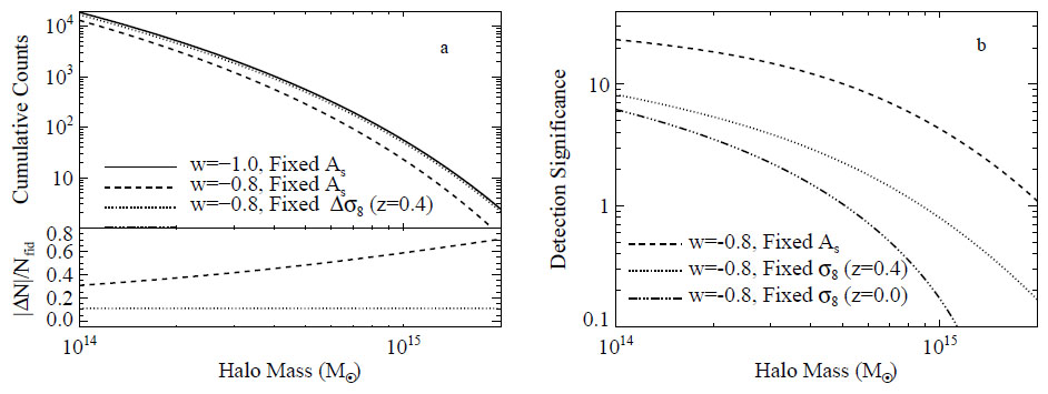 |
Figure 20. (a) Cumulative halo counts as a function of limiting mass for a 104 deg2 survey in a redshift slice z = 0.4± 0.05. The solid line shows the fiducial model from Table 1. The dashed line corresponds to w = -0.8 with the amplitude of the primordial matter power spectrum held fixed. The dotted line has w = -0.8, but holds σ8(z = 0.4) fixed. Residuals relative to the fiducial model are shown in the bottom panel. The small, nearly constant offset of the dotted line is sourced by the dark energy dependence of the comoving volume element dVc. (b) The significance with which this hypothetical halo sample could distinguish the fiducial model from the alternatives in panel (a) as a function of mass threshold, using the statistical error of equation (140). The dot-dashed line shows an additional model in which σ8(z = 0) is held fixed. Even though the high mass end of the halo mass function depends most strongly on cosmology, the statistical power of the cluster abundances is dominated by the low mass end because of the much lower measurement errors. |
While the mean halo abundance becomes more sensitive to σ8(z) at higher masses, the statistical precision with which one can measure σ8(z) decreases with increasing mass because of the larger Poisson fluctuations for rarer clusters. This point is illustrated in Figure 20b, which shows the statistical significance at which a 104 deg2, z = 0.35-0.45 cluster survey would distinguish the models shown in panel (a). For reference, we also show the case in which σ8 is held fixed at z = 0, which reduces model differences because the growth and volume element effects act in opposite directions. We discuss statistical errors in cluster abundances, including the role of sample variance, in Section 6.3.1. The key conclusion from Figure 20b is that lower mass clusters allow stronger model discrimination.
Cluster cosmology requires making an explicit link between the theoretically predicted population of halos as a function of mass and an observed population of clusters. This problem is complicated by the fact that the halo population is usually characterized using dark matter simulations, whereas clusters are identified using baryonically-sourced signatures such as the presence of galaxy overdensities, extended X-ray emission, or SZ decrements (see Section 6.3.2). The lower mass limit probed by cluster abundance experiments is partly set by the detection thresholds intrinsic to each method, but also by the difficulty of characterizing the relation between low mass halos and poor clusters. Different researchers adopt varying definitions of halos and of clusters. Within a reasonable range, such variation is acceptable, provided each study is self-consistent and the halo-cluster relation is accurately characterized. In recent years, numerical studies have mostly shifted from the friends-of-friends algorithm used in earlier work (e.g., Efstathiou et al. 1988) to spherical overdensity definitions (e.g., Tinker et al. 2008), thus avoiding the tendency of the friends-of-friends method to occasionally link distinct mass concentrations via narrow bridges (see More et al. 2011 and references therein for a more detailed discussion). Halo boundaries are typically drawn at overdensities Δ ≈ 100-500, where clusters are in approximate dynamical equilibrium and where mass predictions are fairly robust to baryonic physics. The overdensity Δ can be quoted relative to the mean matter density of the universe at the cluster redshift or relative to the critical density at that redshift. In this section, we will adopt Δ = 200 with respect to the mean density as our definition unless otherwise specified.
The principal challenge to precision cosmology with clusters is not cluster identification per se, but the accurate calibration of the relation between cluster observables (e.g., richness, X-ray luminosity, SZ decrement) and halo masses. Figure 21 illustrates this point by flipping the x and y axes of panel (a) in Figure 20, thus plotting the mass threshold at fixed cluster abundance for the different cosmological models. Changing from w = -1 to w=-0.8 while holding As fixed changed the predicted abundances by 30-60%, but the corresponding change in mass threshold is only about 20%. For fixed σ8(z = 0.4), the 15% change in abundance corresponds to a 2.5%-6% change in mass threshold. These, then, are the levels of accuracy in mass calibration that must be attained to distinguish between the two w = -0.8 models and our fiducial w = -1 model. The issue of mass calibration will arise repeatedly in this section, especially in Section 6.3.3 and Section 6.4.3.
 |
Figure 21. Halo mass thresholds as a function of cumulative number counts, i.e. flipping the x and y axes of Figure 20a. The x-axis shows the number of halos predicted in a 104 deg2 survey in a redshift slice z = 0.4± 0.05. The lower panel shows the fractional change in mass threshold relative to the fiducial cosmological model. |
In principle, cluster abundances are sensitive to σ8(z), Ωm, and the comoving volume element dVc, as well as any inherent sensitivity of the relation between cluster mass and cluster observables on the distance-redshift relations. To simplify our discussion, we will usually assume that a combination of other data sets (CMB, SN, BAO, WL, etc.) will determine both Ωm and dVc(z) at higher precision than that achievable from cluster abundances. Consequently, we will focus on the sensitivity of cluster abundances to σ8(z) while holding Ωm, dVc(z), and the angular and luminosity distances fixed. In practice, we expect our assumption should be a good one as far as the comoving volume element and the distances are concerned. However, the sensitivity attainable with clusters is high enough that holding Ωm fixed may be incorrect in detail. We will discuss this point in Section 6.6 and again in Section 8.4.
Many cluster cosmology papers quote masses in h-1 M⊙ because observational mass estimates (and, to some extent, theoretical predictions) scale inversely with h. However, at non-zero redshift many other parameters also come into play, and h is itself one of the parameters constrained by dark energy experiments. Thus, we have elected to quote masses in M⊙ rather than h-1 M⊙. In a similar vein, we will switch most of our subsequent discussion from σ8 to σ11,abs, the rms fluctuation on a scale of R = 11 Mpc (equal to σ8 for h = 0.727). For some observables (e.g., the X-ray estimated gas mass Mgas, the inferred cluster mass is sensitive to the angular diameter distance DA(z) and this dependence itself provides useful cosmological constraints; this point is discussed by Allen et al. (2011) but we will not address it further here. Our primary focus is the statistical precision with which cluster abundances constrain σ11,abs(z), and the level at which systematic uncertainties must be controlled to achieve these statistical limits. In Section 6.6 we compare the precision potentially attainable with clusters to forecasts (described in Section 8) from fiducial Stage III and Stage IV CMB+SN+BAO+WL programs.
6.2. The Current State of Play
Most cluster cosmology studies of the past decade have been based on X-ray catalogs, with typical cluster samples numbering in the several tens to few hundreds of clusters. The vast majority of these catalogs rely on ROSAT data — either from the ROSAT All-Sky Survey (RASS; Voges et al. 1999) or from serendipitous detections in pointed observations — though there are also samples selected based on XMM-Newton and Chandra imaging. Table 4 summarizes some of the main X-ray catalogs that have been employed in these studies. The recently approved XXL survey will add ≈ 50 deg2 of imaging, contributing ≈ 600 clusters out to z = 1 and above. The next big step forward for X-ray samples is the eROSITA mission, which should identify ≈ 80,000 galaxy clusters at high confidence (see Section 6.5).
| Catalog/Reference | Type of Survey | No. of Clusters | Redshift Limit |
| BCS (Ebeling et al. 2000) | Wide/Shallow | 107 | 0.3 |
| NORAS (Bvhringer et al. 2000) | Wide/Shallow | 378 | 0.3 |
| HIFLUGCS (Reiprich and Bvhringer 2002) | Wide/Shallow | 63 | 0.2 |
| WARPS (Perlman et al. 2002) | Narrow/Deep | 34 | 0.8 |
| SHARC (Burke et al. 2003) | Narrow/Deep | 48 | 0.7 |
| 160 deg2 (Mullis et al. 2003) | Narrow/Deep | 201 | 0.7 |
| REFLEX (Bvhringer et al. 2004) | Wide/Shallow | 447 | 0.3 |
| 400 deg2 (Burenin et al. 2007) | Narrow/Deep | 287 | 0.8 |
| MACS (Ebeling et al. 2010) | Wide/Shallow | 34 | 0.6 |
| MCXC (Piffaretti et al. 2011) | Compilation | 1783 | 0.8 |
| XCS (Lloyd-Davies et al. 2011) | Narrow/Deep | 1022/3669* | 0.8 |
| All cluster catalogs included above are drawn from ROSAT data, except for XCS, which is a serendipitous cluster search in XMM-Newton archival data (see (Mehrtens et al. 2012) for the first data release). Wide/shallow survey catalogs refer to cluster searches in the ROSAT All-Sky Survey (RASS), whereas narrow/deep catalogs are drawn from pointed ROSAT or XMM-Newton observations. MCXC is a compilation of various X-ray cluster catalogs. The characteristic high redshift limit shown is not the redshift of the highest redshift cluster in the sample, but rather a redshift that contains ≳ 90% of the galaxy clusters. The highest cluster redshifts can be significantly higher than the redshift quoted, as expected for flux limited surveys. | |||
| *1022 is the number of galaxy clusters with ≥ 300 photons, allowing for TX estimates. 3669 is the number of 4σ cluster candidates. | |||
The largest existing cluster samples are optically selected, using either spectroscopic or photometric galaxy catalogs. The former benefit from much finer spatial resolution along the line of sight. They tend to be shallow, with typical z ≲ 0.2 (Merchan and Zandivarez 2002, Kochanek et al. 2003, Miller et al. 2005, Merchan and Zandivarez 2005, Berlind et al. 2006, Yang et al. 2007, Li and Yee 2008, Blackburne and Kochanek 2012), though high redshift spectroscopic catalogs do exist (Gerke et al. 2005, Coil et al. 2006). Photometric cluster catalogs hail back as far as the original Abell (1958) catalog, which contained upwards of 2500 systems and served as the primary basis of cluster studies for decades. Though many recent photometric catalogs have focused on narrow but deep survey data (z ≲ 1, e.g., Gonzalez et al. 2001, Gladders and Yee 2005, Milkeraitis et al. 2010, Adami et al. 2010), the SDSS has led to the publication of several moderately deep (z ≲ 0.5) and wide catalogs, which can contain upwards of 50,000 clusters (e.g. Koester et al. 2007, Wen et al. 2009, Hao et al. 2010, Szabo et al. 2011). Extensions that reach out to z ≈ 1 over 1000 deg2 or more from current or near future photometric surveys — such as RCS-2, DES, Pan-STARRS, and HSC — will expand samples to the hundreds of thousands.
One limiting factor that affects these optical cluster finding experiments is that the 4000 E break in the spectrum of early-type galaxies shifts into the near-IR at z ≈ 1, making optical detection challenging above this redshift. This difficulty can be overcome with IR adaptations of optical cluster finding techniques. Today, there are two independent efforts aiming to detect galaxy clusters using IR data: the IRAC Shallow Cluster Survey (ISCS; Eisenhardt et al. 2008) and the Spitzer Adaptation of the Red-Sequence Cluster Survey (SpARCS; Wilson et al. 2006). Both surveys have discovered and spectroscopically confirmed candidate galaxy clusters out to redshift z ≲ 1.5 (e.g., Stanford et al. 2005, Brodwin et al. 2006, Eisenhardt et al. 2008, Muzzin et al. 2009, Wilson et al. 2009, Demarco et al. 2010), with some recent detections reaching z ≲ 2 (Stanford et al. 2012, Zeimann et al. 2012). Additionally, some of these systems have also been detected in X-rays and/or SZ (Brodwin et al. 2011, Andreon and Moretti 2011, Brodwin et al. 2012). These early results are encouraging and suggest that IR detection of high redshift clusters can play an important role in the future of cluster cosmology.
While detections of the SZ effect in known galaxy clusters date back as early as 1976 (Gull and Northover 1976), it is only recently that instrumentation advances have made large scale SZ searches feasible. The first three successful cluster SZ surveys — using the South Pole Telescope (SPT), the Atacama Cosmology Telescope (ACT), and the Planck satellite — are all currently ongoing. All three projects have released SZ-selected cluster samples (Vanderlinde et al. 2010, Marriage et al. 2011, Planck Collaboration et al. 2011a, Williamson et al. 2011, Reichardt et al. 2013). These samples tend to be of very massive clusters (see Figure 27) and, in the case of ACT and SPT, extend to z ≈ 2, with the upper limit set by the lack of massive galaxy clusters above this redshift. For ACT and SPT, this redshift coverage is limited only by the abundance of such massive objects at high redshift. Planck is limited in part by its relatively large beam, but it has the important benefit of being an all sky survey, which results in a larger cluster yield overall. Based on the sensitivity estimates shown in Figure 27 below, we anticipate ~ 700 clusters in 2500 deg2 for SPT and ~ 11,000 over the full sky for Planck. We emphasize, however, that these numbers can easily shift by factors of ~ 2-3 depending on the signal-to-noise cut adopted for cluster identification. In contrast to optical and X-ray techniques, there is not likely to be a major leap forward in SZ capabilities in the next few years, so the SPT, ACT, and Planck samples will probably remain the largest SZ cluster samples available for the next decade. That said, the limiting masses of SZ cluster samples will go down as these and other facilities conduct deeper surveys focused on CMB polarization (e.g., ACTPol and SPTPol).
Existing cluster cosmology constraints have come primarily from X-ray data (see, e.g., Henry 2000, Reiprich and Bvhringer 2002, Schuecker et al. 2003, Allen et al. 2003, Pierpaoli et al. 2003), reflecting the fact that X-ray observables can be related to mass via simulations and/or analytic approximations and by hydrostatic modeling for well observed clusters. All three of the most recent X-ray analyses yielded tight, consistent cosmological constraints, which can be summarized as σ8(Ωm / 0.25)0.45 = 0.80 ± 0.03 (Henry et al. 2009, Vikhlinin et al. 2009, Mantz et al. 2010). Cosmological analyses from optical samples have typically been less constraining because of uncertain mass calibration (see, e.g., Bahcall et al. 2003, Gladders et al. 2007, Wen et al. 2010). However, recent work that uses stacked weak lensing analysis for mass calibration (Johnston et al. 2007, Mandelbaum et al. 2008, Sheldon et al. 2009) has allowed optical samples to achieve the same level of precision as X-ray samples (Rozo et al. 2010), with comparable levels of systematic error. Constraints from SZ selected samples are emerging (Vanderlinde et al. 2010, Sehgal et al. 2011, Reichardt et al. 2013), and while they are currently weak because of the relatively large uncertainty in the SZ-mass scaling relation, the extensive follow-up campaigns that are currently underway will reduce this scaling uncertainty and bring these constraints to a level comparable to those from optical and X-ray cluster catalogs (e.g. High et al. 2012, Hoekstra et al. 2012, Planck Collaboration 2012, Rozo et al. 2012d).
Regardless of the wavelength of choice, current cluster abundance constraints are limited not by the number of clusters but by uncertainty in mass calibration. Figure 22 shows the cluster abundance constraints from several recent analyses. Because the current X-ray and optical mass calibrations are fundamentally different (hydrostatic vs. weak lensing), the excellent agreement illustrated in Figure 22 provides a strong test of systematic uncertainties. However, the results from the (Planck Collaboration et al. 2011b) have sounded a cautionary note, as the optical mass estimates used to derive cosmological parameters in Rozo et al. (2010) appear to be inconsistent with SZ data (see also Draper et al. 2012). Biesiadzinski et al. (2012) have attributed this inconsistency to miscentering, while 2012Angulo et al. point out the importance of systematics covariance. Rozo et al. (2012c, 2012b, 2012a) argue that the optical, X-ray, and SZ data can be reconciled by considering, in addition to these effects, the systematics of X-ray temperature measurements indicated by the offsets among estimates from different groups, and departures from hydrostatic equilibrium at the level predicted by hydrodynamic cosmological simulations (e.g., Nagai et al. 2007). Regardless of how this issue is ultimately resolved, it is clear that further tightening cosmological constraints will require a significant improvement in our ability to estimate cluster masses.
 |
Figure 22. Comparison of the 68% confidence regions derived from galaxy cluster abundances and WMAP CMB data by various groups. The first three error ellipses — using quoted uncertainties from Mantz et al. (2010), Henry et al. (2009), and Vikhlinin et al. (2009) — all come from X-ray selected cluster samples. The Rozo et al. (2010) ellipse comes from an optically selected cluster sample with stacked weak lensing mass calibration. The Tinker et al. (2012) constraint uses the same optical clusters and mass calibration, but relies on galaxy clustering and mass-to-number ratios to derive cosmological constraints, making it essentially an independent cross-check. The Benson et al. (2011) ellipse comes from the SPT selected cluster sample. |
On this last count, we note that Figure 22 also includes cosmological constraints from an analysis by Tinker et al. (2012) that does not rely on cluster abundances. Tinker et al. (2012) use a halo occupation model (see Section 2.3) fit to SDSS galaxy clustering, which yields a prediction for the mass-to-number ratio of clusters 66 as a function of σ8 and Ωm. While this analysis uses the same weak lensing mass calibration as Rozo et al. (2010), the method is less sensitive to the mass scale and is entirely independent of abundance uncertainties, making it a largely independent measurement and a powerful systematics cross-check. The same approach can be adapted to future, deeper photometric surveys. We also note that stacked weak lensing measurements for clusters can be extended far beyond the virial radius Sheldon et al. (2009), into the regime where they measure the large scale cluster-mass cross-correlation function, and that these large scale measurements can also be used to constrain cosmological parameters (Zu et al. 2012).
6.3. Observational Considerations
6.3.1. Expected Numbers and Cosmological Sensitivity
Figure 23a shows the expected cluster counts in our fiducial cosmological model for a variety of limiting masses, as a function of the limiting redshift z of a 104 deg2 survey. (Note that these are lower limits on mass but upper limits on redshift.) Panel (b) shows number counts in redshift bins of width ± 0.05; e.g., at z = 0.15, we show the halo counts in the redshift bin [0.1,0.2]. We maintain this redshift binning convention throughout. Together, these two figures give a broad-brush sense for the typical sample sizes and redshift distribution of galaxy clusters as a function of limiting mass and redshift.
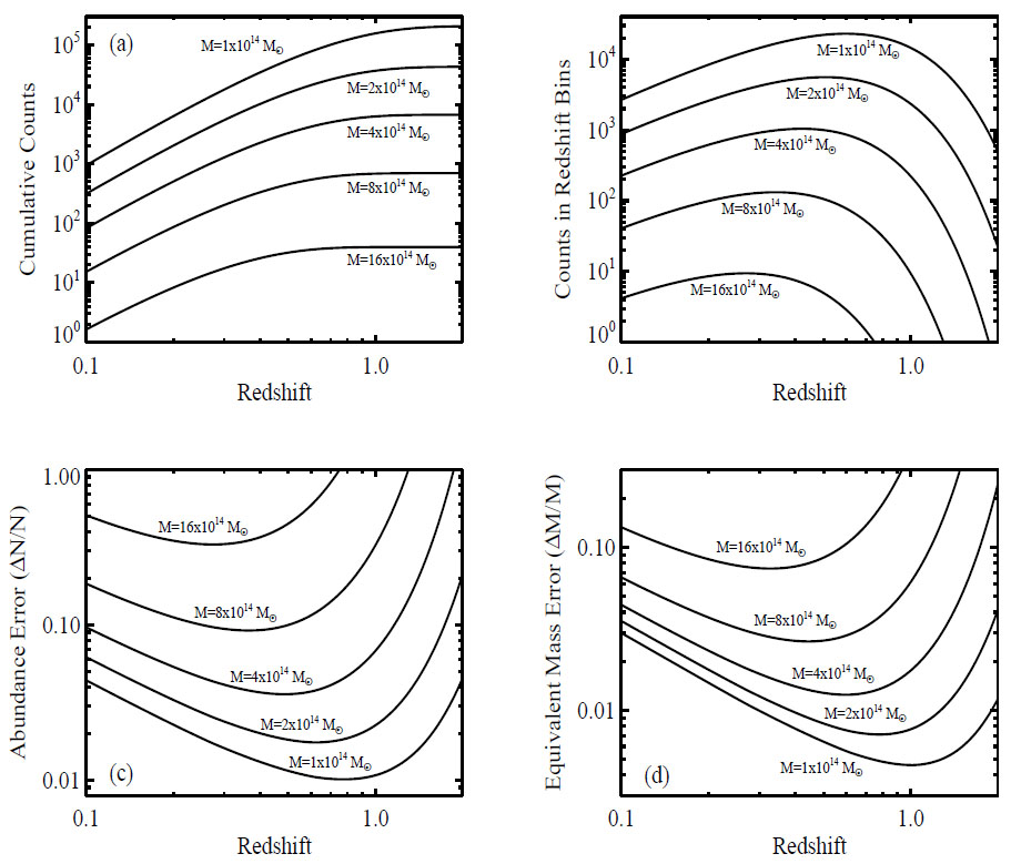 |
Figure 23. (a) Cumulative halo number counts above the indicated mass thresholds M as a function of the limiting survey redshift. We assume the fiducial cosmological model from Table 1, and survey area of 104 deg2. (b) Counts above the mass threshold in redshift bins z = zc ± 0.05. (c) Statistical error in the number of clusters above the mass threshold from equation (140), again in redshift bins z = zc ± 0.05. (d) The mass accuracy required to ensure that cosmological constraints are limited by the statistical precision in the number of galaxy clusters rather than by uncertainties in mass estimation. |
Assuming halo masses can be adequately measured, the statistical error in cluster abundances is the sum in quadrature of Poisson noise and sample variance (Hu and Kravtsov 2003),
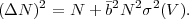 |
(140) |
Here, N is the mean number of halos in the volume of
interest,  is the mean
bias of the halos, and
σ2(V) is the variance of the matter density
field over the survey volume.
67
Figure 23c shows the fractional error
ΔN / N
for the fiducial model, again for redshift bins z =
zc± 0.05 where zc is
the central redshift of the bin.
Sample variance becomes larger than Poisson variance below a transition mass
~ 4 × 10¹⁴
M⊙ at z = 0.1 and ~ 1014
M⊙ at z = 1.
However, the statistical error is never more than a factor ~ 2
above the N-1/2 Poisson expectation (see
Figure 26 below),
and total statistical errors should scale with survey area roughly as
(A / 104 deg2)-1/2.
For any mass threshold the statistical error first
decreases with redshift, as the number of clusters grows with the increasing
comoving volume per Δz.
This trend flattens when the clusters become exponentially
rare, at which point further increase in redshift leads to a precipitous
drop in the number of clusters and a corresponding rise in Poisson
errors. These competing effects lead to
the characteristic U-shape of the curves in
Figure 23c.
is the mean
bias of the halos, and
σ2(V) is the variance of the matter density
field over the survey volume.
67
Figure 23c shows the fractional error
ΔN / N
for the fiducial model, again for redshift bins z =
zc± 0.05 where zc is
the central redshift of the bin.
Sample variance becomes larger than Poisson variance below a transition mass
~ 4 × 10¹⁴
M⊙ at z = 0.1 and ~ 1014
M⊙ at z = 1.
However, the statistical error is never more than a factor ~ 2
above the N-1/2 Poisson expectation (see
Figure 26 below),
and total statistical errors should scale with survey area roughly as
(A / 104 deg2)-1/2.
For any mass threshold the statistical error first
decreases with redshift, as the number of clusters grows with the increasing
comoving volume per Δz.
This trend flattens when the clusters become exponentially
rare, at which point further increase in redshift leads to a precipitous
drop in the number of clusters and a corresponding rise in Poisson
errors. These competing effects lead to
the characteristic U-shape of the curves in
Figure 23c.
Figure 23d converts these statistical abundance errors to equivalent errors in mass by dividing ΔN / N by the logarithmic slope of the cumulative halo mass function, α= - d lnN / d lnM, which ranges between 2 and 5 depending on redshift and mass. While observational samples are not thresholded exactly in mass, the sensitivity of cluster abundances to an overall shift in the mean mass at fixed observable is well captured by this heuristic argument. In order for clusters to saturate the statistical limit in the abundances, the uncertainty in mass calibration must be smaller than this ΔM / M. For a 104 deg2 survey and M ≥ 8 × 10¹⁴ M⊙, a mass accuracy of 3%-10% (depending on z) suffices. By M≈ 2 × 10¹⁴ M⊙, however, the accuracy requirement has sharpened to ≲ 1%. (This last number agrees well with the more detailed analysis of Cunha and Evrard (2010) for a mass threshold of 1014.2 M⊙; see in particular the top panels in their Figure 2.) Achieving such accuracy is a tall order, and current studies are clearly limited by the systematic uncertainty in cluster masses rather than abundance statistics. Note that the required accuracy scales roughly as (A / 104 deg2)-1/2, and it applies to the overall mass scale (i.e., the mean of the mass-observable relation) rather than the mass of any individual system.
Figure 24 translates the errors on cluster abundance from Figure 23 to errors on the matter power spectrum amplitude σ11,abs(z), again for a 104 deg2 survey with z = zc ± 0.05 bins. For simplicity, we assume that Ωm, the comoving volume element dVc(z), and the power spectrum shape are perfectly known from independent data (CMB+SN+BAO+WL), so that σ11,abs(z) is the single cosmological parameter controlling the cluster abundance. As discussed in Section 6.1, if the uncertainty in Ωm is non-negligible, then it is the combination σ8(z) Ωmq that is constrained instead. Panel (a) shows the case where mass calibration errors are negligible. The errors on σ11,abs(z) roughly track the abundance errors ΔN / N in Figure 23, but because the sensitivity of the abundance to σ11,abs(z) at fixed mass increases with increasing redshift, the best constraint on σ11,abs(z) comes at a higher redshift than the one at which ΔN/N is minimized. The remaining panels show the impact of 1%, 2%, 4%, and 8% mass calibration errors for three different threshold masses.
 |
Figure 24. Statistical error on σ11,abs(z) as a function of redshift, in redshift bins z = zc ± 0.05, for different mass thresholds as labeled. We assume a 104 deg2 survey area, and the fiducial cosmological model. We also assume that Ωm, the shape of the matter power spectrum, and the comoving volume element dVc are perfectly known from independent data (CMB+SN+BAO+WL). Panels (b)-(d) refer to specific mass thresholds as labeled. In each panel the solid curves show the effect of different mass calibration uncertainties as labeled while the dotted curve assume the perfect mass calibration values (i.e., number statistics limited) from panel (a). For reference, the uncertainty in σ11,abs(z) that we forecast for a fiducial CMB+SN+BAO+WL program is ~ 1% for Stage IV data sets and ~ 2-3% for Stage III data sets (see Section 6.6 and Section 8.4). |
The basic features in Figure 24 are simple to understand at a quantitative level, starting from the knowledge that cluster abundances constrain the combination σ11,abs(z) Ωmq with q ≈ 0.4. Since the mass of a collapsed volume scales linearly with Ωm, a shift of the mass scale by a constant factor is nearly degenerate with a change of Ωm by the same factor. Together these scalings imply σ11,abs(z) ∝ Mq, where M is the mass scale at fixed abundance, making Δlnσ11,abs(z) ≈ q Δ lnM for a survey limited by mass calibration uncertainty ΔlnM. For a survey limited by halo statistics, the corresponding effective mass error is (ΔlnM)eff = α-1 ΔlnN where α= - dlnN / dlnM ≈ 2-5 is the slope of the cumulative halo mass function, so in this case Δlnσ11,abs(z) ≈ q α-1 ΔlnN. Combining the two limits we arrive at
 |
(141) |
The above expression fits the data in Figure 24 with better than 30% accuracy (typically ≲ 15%).
Figure 25 plots the value of the degeneracy exponent q as a function of limiting mass and redshift. In the Press-Schechter (Press and Schechter 1974) theory of the halo mass function, the cumulative abundance is set by the probability that a point in a Gaussian field of variance σ2(M) exceeds the critical threshold δc ≈ 1.69 for spherical collapse (see Section 2.3), so that N ∝ [1 - erf(δc / √2 σ(M)) ]. Putting in the σ(M, z) relation for a ΛCDM power spectrum yields a logarithmic derivative dlnN / dlnσ ≡ ασ≈ 5-9 depending on mass and redshift. Because cluster abundances are degenerate in Ωm / M, the logarithmic derivative of cluster abundances relative to Ωm is the same as the slope α of the mass function (but with opposite sign), so locally the cumulative mass function scales as
 |
(142) |
We see that halo abundances are degenerate in σ11,abs(z) Ωmq with q = -α / ασ ≈ 3/7 ≈ 0.4. We plot the ratio α / ασ — computed using the Tinker et al. (2008) mass function rather than the Press-Schechter mass function — in Figure 25.
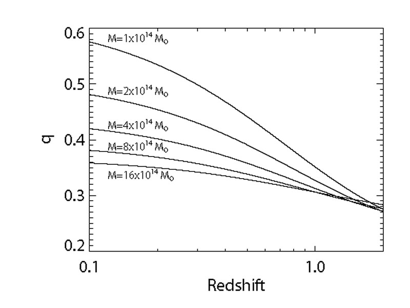 |
Figure 25. The degeneracy exponent q as a function of redshift for a series of threshold masses. The parameter q is the exponent in σ11,abs(z) Ωmq that holds the abundance of galaxy clusters above the quoted threshold mass at the appropriate redshift bin fixed for small, oppositely directed changes in σ11,abs(z) and Ωm. |
A cluster abundance analysis becomes limited by mass scale uncertainty rather than halo abundance statistics when ΔlnM > α-1 ΔlnN. If we approximate the error as Poisson, ΔlnN = N-1/2, then an experiment is limited by mass uncertainty if the sample size is N ≥ (α ΔlnM)-2. Current systematic uncertainties in mass calibration are ≈ 10%, which for α ≈ 3 corresponds to N ≈ 10. Thus, cluster abundance studies are limited by uncertainty in the overall mass scale even for samples with as few as ≈ 10-20 galaxy clusters. For cluster samples with N ≈ 103 (104), the accuracy required in mass estimation for an experiment to be dominated by halo statistics is ≈ 1% (0.3%). So that one may apply the rule-of-thumb estimates derived in this section, Figure 26 plots the mass-function slope α and the ratio of the total error ΔlnN to the Poisson uncertainty N-1/2. Note that abundance errors including sample variance almost never exceed twice the Poisson error and are often much closer. Using Figures 25 and 26 along with equation (141), one can quickly estimate how well an experiment with given number of galaxy clusters N can constrain σ11,abs(z).
 |
Figure 26. Left: Logarithmic derivative α = -dlnN / dlnM of the cumulative halo counts, as a function of redshift, for five mass thresholds as labeled. Right: The ratio of the total (Poisson + sample variance) error in the halo counts ΔlnN to the Poisson error N-1/2. Solid lines assume a survey area of 10,000 deg2, while dashed lines correspond to 100 deg2. In conjunction with Fig. 25 and equation (141), these figures allow one to quickly estimate how well σ11,abs(z) can be constrained at each redshift by a galaxy cluster sample with N clusters. |
If Ωm and dVc(z) are not perfectly known, then cluster abundances will constrain a combination of cosmological parameters rather than the matter fluctuation amplitude alone. Predicted abundances are proportional to dVc(z), so for an experiment dominated by uncertainty in the mass scale, uncertainty in the volume element will affect the interpretation if ΔlndVc ≳ α ΔlnM, the effective abundance uncertainty. SN and BAO surveys should typically yield uncertainties below this limit, so we expect regarding dVc(z) as known to be an adequate approximation for our purposes, though it may fail for sufficiently powerful cluster surveys. Since a pure shift in Ωm is equivalent to a shift in mass scale, uncertainties in Ωm are relevant if ΔlnΩm ≳ ΔlnM, where we have again assumed the experiment in question is dominated by the mass error ΔlnM. If the uncertainty in Ωm is larger than this critical scale, then clusters will effectively constrain σ11,abs(z) Ωmq rather than σ11,abs(z) alone. Equation (141) will still hold, but one must replace Δlnσ11,abs(z) by Δln[ σ11,abs(z) Ωmq ]. Current fractional uncertainties in Ωm from CMB and other observables are ~ 10%, comparable to mass calibration systematics. Future studies will reduce Ωm uncertainties, but they may remain significant compared to improved mass calibration errors in cluster surveys.
We have focused our discussion here on cumulative cluster abundances — i.e., space densities of clusters above a mass threshold — while observational analyses usually examine the differential distribution as a function of observable mass-proxies. Differential distributions are useful for breaking degeneracies (e.g., among σ11,abs, Ωm, and dVc), and for constraining "nuisance parameters" such as the scatter of the observable-mass relation. However, for single-parameter constraints on σ11,abs(z), we expect that our analysis of the cumulative abundance uncertainties provides an accurate guide, as it makes use of the single number best determined by the data for any given mass threshold and redshift range. We anticipate that observational analyses will continue to concentrate mainly on differential distributions, but cumulative distributions are more amenable to the kind of rule-of-thumb estimates that we try to develop throughout this section, so they provide a more intuitive way of understanding the cosmological information content of cluster surveys.
Each of the three main methods for finding galaxy clusters — optical, X-ray, and SZ — has its own virtues and deficiencies. The principal advantage of optical surveys is sheer statistics, reflecting the low mass threshold for optical detection; clusters with masses as low as 5 × 10¹³ M⊙ are capable of hosting significant galaxy overdensities. Near-future surveys (RCS-2, DES, HSC, Pan-STARRS) should find ≈ 105 systems in areas of 103-104 deg2 out to z ≈ 1. On a longer time scale (≈ 10 years), surveys with LSST should increase the available cluster samples by another factor of 5-10, due both to larger area (≈ 20,000 deg2) and to deeper imaging, which should allow cluster detection out to z ≈ 1.5. Finally, cluster searches in the IR are capable of finding galaxy clusters out to z ≈ 2, but large survey areas to this depth will only be achievable with the advent of Euclid and/or WFIRST. With the stacked weak lensing mass calibration that we advocate in Section 6.3.3, the calibration accuracy scales with cluster number as N-1/2, so enormous samples are statistically advantageous even if mass uncertainties dominate the error budget.
The main drawback for optical cluster detection is projection effects, i.e., chance alignments of multiple low mass halos along the line of sight that are misidentified as a single massive galaxy cluster. While this systematic has been drastically suppressed in modern surveys with multi-band photometry and photometric redshift estimators, one still expects 5%-20% of photometrically selected clusters to suffer from serious projection effects (Cohn et al. 2007, Rozo et al. 2011a). The importance of projection effects increases with decreasing mass, so we expect it is projection effects rather than survey depths that will ultimately set the detection mass threshold for optical cluster finding in future surveys.
Unlike optical studies, X-ray cluster searches are nearly free from projection effects. This robustness to the presence of structures along the line of sight reflects the fact that X-ray emission scales as density-squared, which enhances the relative contrast of a cluster in the sky, and it is the principal reason that X-rays are considered the cleanest method for selecting galaxy clusters. The main difficulty for X-ray selection is a technological one, specifically, the need for space-based observatories. A dramatic leap forward in capabilities will happen with the launch of eROSITA, which should detect ≈ 105 galaxy clusters over the full sky out to z = 1 and beyond, ensuring that X-rays will continue to play a critical role in the development of cosmologically relevant cluster samples over the coming decade. On a longer time scale, further improvements would require X-ray observatories that reach lower flux limits with higher angular resolution, both of which are needed to detect large numbers of systems at z ≳ 1.
The primary advantage of SZ searches is that they do not suffer from cosmological dimming. The SZ signature arises from up-scattering of CMB photons by the hot intra-cluster plasma, and because the number of up-scattered photons does not depend on the distance to the cluster the signal is roughly redshift independent. In practice, the SZ signal is not exactly redshift independent because of residual sensitivity to the relative size of the cluster and the beam of the telescope. Unfortunately, achieving sufficient sensitivity to detect low mass clusters in SZ is technologically very challenging. For instance, the current SPT, ACT, and Planck surveys are expected to be complete at all redshifts above mass thresholds of 7 × 10¹⁴ M⊙, 1015 M⊙, and 2 × 10¹⁵ M⊙ respectively (Vanderlinde et al. 2010, Marriage et al. 2011, Planck Collaboration et al. 2011a); while these limits will go down, they will not reach thresholds comparable to those of X-ray or optical cluster selection. Consequently, while these experiments are currently the best avenue to probe the z ≈ 1 massive cluster population, on a 3-5 year time scale the focus of cluster detection is likely to shift towards optical and X-ray. To our knowledge, there are no current plans to develop a new generation of SZ survey instruments that would dramatically improve upon the capabilities of current experiments for cluster detection, at least compared to the differences in optical (e.g., DES vs. SDSS) and X-ray (eROSITA vs ROSAT). However, both SPTpol and ACTpol should lead to significantly lower mass thresholds for SZ cluster detection than the current SPT and ACT cluster samples.
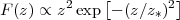
Figure 27 showcases the difference of the cluster populations from the various selection methods, where we have limited ourselves to wide surveys (1000 deg2 or higher) and have shown only a handful of representative selection functions. The top row shows the selection functions for existing or ongoing surveys, while the bottom-row shows the selection for future surveys. The left panels shows the limiting mass as a function of redshift for each of the surveys considered, while the right panels shows the number above the limiting mass in a redshift bin of width Δz = 0.1, accounting for survey area. We emphasize that in practice cluster samples never have a sharp mass threshold; the curves shown in Figure 27 are only roughly indicative of the mass and redshift ranges probed. The number of clusters detected depends in detail on the selection cuts applied, and small changes in threshold translate to larger changes in abundance, so factor-of-two deviations from the projections in Figure 27 would not be particularly surprising.
For the optical detection threshold we have assumed that projection effects limit useful cluster catalogs to a minimum richness λ = 15 in the algorithm of Rykoff et al. (2012), which counts galaxies of luminosity L ≥ 0.2L*. To account for mass-richness scatter, we choose an effective mass threshold that yields approximately the same space density as this richness threshold. The sharp upturn occurs when 0.2L* matches the magnitude limit of the survey. In SZ, we see that the SPT mass threshold (kindly provided by the SPT collaboration, and normalized to a total cluster yield of ≈ 700 clusters at full depth) is only mildly sensitive to redshift. The gentle decrease in limiting mass with increasing z reflects the fact more distant clusters subtend smaller angles that better match the SPT beam size, and that clusters are hotter at fixed mass with increasing redshift. For Planck, conversely, the decreasing angular size of clusters reduces sensitivity at higher redshift because the beam itself is large. The curve shown is a rough estimate of the Planck Early SZ sample (Planck Collaboration et al. 2011a), though the final selection will go considerably lower in mass, because of both deeper data and lower S/N cuts. The SPTpol curve is similar to SPT, but it reaches lower masses over a smaller area, while the ACTpol curve reaches similar noise levels to SPT (≈ 20 μK, Niemack et al. 2010) over a larger area. (ACTpol also plans a separate survey, deeper and narrower than SPTpol.) Turning to X-rays, the REFLEX, XXL, and eROSITA curves all show the increase of mass threshold with redshift characteristic of flux-limited surveys. The XXL selection is that of Valageas et al. (2011) scaled to match the observed density of C1 clusters in the XMM-LSS field (Pacaud et al. 2007), while the eROSITA threshold represents a flux limit ≈ 4 × 10-14 erg s-1, corresponding to ≈ 50 photon counts (Pillepich et al. 2012). The mass limit is higher by a factor of ≈ 3 for clusters reaching 300 photon counts.
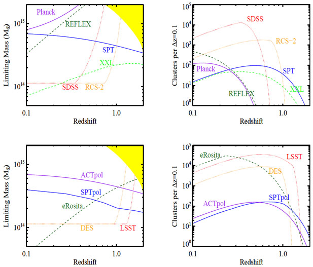 |
Figure 27. Selection function for several representative cluster samples, as labelled. The top panels show surveys that are completed or currently ongoing. The bottom panels show future surveys. Left panels show the limiting mass as a function of redshift, while right panels show the number of galaxy clusters above the limiting mass in redshift bins of width Δz = 0.1. The yellow region in the left panels corresponds to the area in parameter space where one expects fewer than one galaxy cluster above the mass and redshift under consideration. For the abundance plot, we consider the appropriate area for each of the surveys: 30,000 deg2 for the eROSITA and Planck cluster samples, 10,000 deg2 for the REFLEX sample, 20,000 deg2 for LSST, 10,000 deg2 for SDSS, 5,000 deg2 for DES, 1,000 deg2 for RCS-2, 2500 deg2 for SPT, 600 deg2 for SPTpol, and 4000 deg2 for ACTPol. The current ACT survey (not plotted) is similar to SPT, with a somewhat higher mass threshold and a 1000 deg2 survey area. Different line types are used only to aid visual discrimination. |
Current wide X-ray samples are largely limited to massive systems at moderate redshifts, but narrow/deep samples reaching z ≈ 1 and above do exist. By comparison, the SDSS reaches lower mass over large areas of the sky, but it only extends to z ≈ 0.5. RCS-2 reaches z ≈ 1, but over a smaller (though still quite significant) area. The Planck SZ survey is largely limited to massive, moderate redshift systems, while the SPT SZ survey has the best current sensitivity to high redshift clusters. In the near future, DES will extend the range of optical identification to z ≈ 1 over a large area, but eROSITA should ultimately produce a larger sample. While DES has a lower mass threshold over the range 0.3 < z < 1, the larger (all-sky) area of eROSITA leads to a larger cluster total, and eROSITA should continue to detect clusters at z>1 where the DES sensitivity declines rapidly. On a longer time scale, LSST will push the optical selection limit to z ≈ 1.5, increasing the number of z > 1 galaxy clusters by one to two orders of magnitude.
Another proposed method for detecting galaxy clusters is to search for peaks in the weak lensing shear field. However, while massive halos produce local shear peaks, shear peak statistics are known to suffer from severe projection effects: many peaks arise from the superposition of multiple halos along the line of sight. Consequently, shear peak selection is not a particularly effective method for selecting clusters of galaxies. That said, the shear peak abundance is an observable that can be predicted from numerical simulations in much the same way as the halo mass function, and this approach may well yield useful cosmological constraints (e.g., Marian et al. 2009, Dietrich and Hartlap 2010). For the remainder of this review, however, we focus on abundances of clusters identified by optical, X-ray, or SZ methods. We emphasize that stacked weak lensing mass calibration of clusters identified by other methods is not equivalent to shear peak statistics, since cluster methods use the additional information afforded by baryonic density peaks to drastically reduce the impact of projection effects on cluster selection.
6.3.3. Calibrating the Observable-Mass Relation
The biggest challenge for cluster cosmology is characterizing the observable-mass relation P(X|M, z), where X is a cluster observable that is correlated with mass (e.g., richness, YSZ, LX) and P(X|M, z) is the probability that a halo of mass M at redshift z is detected as a cluster with observable X. This relation is usually described by parameters that specify the mean relation, the rms scatter, and perhaps a measure of skewness or kurtosis, all of which can evolve with redshift. There are three general approaches to determining these parameters: simulations, direct calibration, and statistical calibration.
In the simulation approach, one relies on numerical simulations to calibrate the observable-mass relation (e.g. Vanderlinde et al. 2010, Sehgal et al. 2011). The main difficulty that simulation methods face is our incomplete understanding of baryonic physics, particularly galaxy formation feedback processes. These difficulties can be minimized by defining new X-ray observables that are expected to be robust to these details, and through careful exploration of the sensitivity of the observable-mass relation to the physics that goes into the simulations (e.g., Nagai et al. 2007, Rudd and Nagai 2009, Stanek et al. 2010, Fabjan et al. 2011, Battaglia et al. 2012). The simulations themselves are steadily improving thanks to increased computer power, more sophisticated algorithms, and the availability of better data to test the input physics. Despite these trends, we think it unlikely that simulations will achieve the ~ 0.5-2% level of accuracy required for cluster abundance experiments to become statistics dominated in the next ten years.
The second approach to calibrating the observable-mass relation is the direct method, in which a small subset of galaxy clusters have X-ray hydrostatic mass estimates and/or weak lensing mass estimates that are taken to represent "true" masses. The observable-mass relation is directly calibrated on this small subset of galaxy clusters, then applied to the general cluster population (Vikhlinin et al. 2009, Mantz et al. 2010). Unfortunately, hydrostatic mass estimates are themselves problematic because non-thermal pressure support (bulk motions, magnetic fields, cosmic rays) is expected to bias them at the ≈ 10%-20% level (Lau et al. 2009, Meneghetti et al. 2010), and it is not clear that these biases can be predicted at the required level of accuracy. We therefore suspect that hydrostatic estimates will play a steadily decreasing role in future cluster abundance experiments. Weak lensing mass estimates of individual clusters can in principle be unbiased in the mean, but they are typically available only for the most massive galaxy clusters in a given sample because of limited signal-to-noise ratio. In addition, even if the WL shape noise is small, halo orientation and large scale structure introduce irreducible noise in the mass estimates of individual clusters at the 20%-30% level (Becker and Kravtsov 2011). Nonetheless, ambitious efforts to achieve accurate weak lensing masses for substantial samples (≈ 50) of X-ray or SZ-selected clusters are likely to play a key role in improving cluster cosmological constraints over the next few years (Hoekstra et al. 2012, von der Linden et al. 2012).
The final approach to calibrating the observable-mass relation is statistical: instead of relying on precise mass estimates of a subsample of galaxy clusters, the relation is calibrated using additional observables for the full sample that correlate with mass. One such statistical method uses the spatial clustering of the clusters themselves, as characterized by the variance of counts-in-cells (Lima and Hu 2004) or by the cluster correlation function or power spectrum (Schuecker et al. 2003, Majumdar and Mohr 2004, Hütsi and Lahav 2008). Because the bias of halo clustering depends on mass (Figure 1), the amplitude and scale-dependence of clustering provides information about the mass-observable relation. Operationally, one parameterizes this relation, then uses standard likelihood methods to jointly fit for both cosmology and the P(X|M, z) parameters (Hu and Cohn 2006, Holder 2006). These types of analyses are often referred to as "self-calibration" because they do not require "direct" mass calibration data. However, we think the descriptor "statistical mass calibration" is more accurate.
The other statistical method we consider is stacked weak lensing, wherein one measures the mean tangential shear of background galaxies around galaxy clusters in a bin of fixed observable. In other words, the stacked weak lensing signal is the cluster-shear correlation function, which can be inverted to yield the mean 3-d mass profile of clusters in the bin (Johnston et al. 2007). Because this measurement allows one to stack many clusters, one can easily obtain high signal-to-noise measurements even for low mass clusters and large angular distances (Mandelbaum et al. 2008, Sheldon et al. 2009). Since the underlying halo population is randomly oriented relative to the line of sight, stacked weak lensing mass calibration does not suffer from orientation biases so long as the cluster identification itself does not preferentially select halos oriented along a particular direction or aligned with line-of-sight structure. However, orientation biases in the cluster selection method will probably exist to some degree, and they must be calibrated carefully on simulations. Finally, because this method relies on stacking all galaxy clusters, it only provides information about the mean of the mass-richness relation, so additional data are required to provide tight constraints on the scatter. 68
Figure 28 shows the error in mass calibration
that can be
achieved using stacked weak lensing for both "Stage III" (left panel) and
"Stage IV" (right panel) observations, calculated via the methodology
described by
Rozo et
al. (2011b).
Briefly, we assume a source redshift distribution
appropriate for DES-like survey depth, and we sum over all annuli within
the radius 2R200, which is a rough approximation for
the location of the one-to-two halo transition of the matter correlation
function using the
Hayashi and White
(2008)
model. (Other studies, e.g.
Tavio et
al. 2008,
also find that one-halo regime of the mass profile
extends well beyond R200.)
For our Stage III estimates we assume an intrinsic shape noise
σe = 0.4 and
source galaxy surface density
 g = 10
arcmin-2, while for Stage IV we assume
σe = 0.3 and
g = 30
arcmin-2.
Note that the corresponding tangential shear error is
σγ
≈ σe /
√2.
These values correspond roughly to expectations for
DES data and Euclid/WFIRST data, respectively;
the lower σe for the latter reflects higher image
quality, though the partition of this improvement between
σe
and g is
somewhat arbitrary. LSST falls between these two cases but closer to
Stage IV. We assume that clusters have NFW mass profiles
(Navarro et
al. 1996),
and we include the decrease
in background source density with increasing cluster redshift.
In all cases, the redshift distribution is set to
g = 10
arcmin-2, while for Stage IV we assume
σe = 0.3 and
g = 30
arcmin-2.
Note that the corresponding tangential shear error is
σγ
≈ σe /
√2.
These values correspond roughly to expectations for
DES data and Euclid/WFIRST data, respectively;
the lower σe for the latter reflects higher image
quality, though the partition of this improvement between
σe
and g is
somewhat arbitrary. LSST falls between these two cases but closer to
Stage IV. We assume that clusters have NFW mass profiles
(Navarro et
al. 1996),
and we include the decrease
in background source density with increasing cluster redshift.
In all cases, the redshift distribution is set to
 |
(143) |
with z* = 0.5. This is appropriate for DES and underestimates the redshift depth for LSST, which will result in a slight overestimate of the statistical uncertainties for Stage IV experiments, particularly at the highest redshift bins.
In each panel of Figure 28, dashed red curves show the error from shape noise alone, while solid curves include the intrinsic scatter between noiseless WL mass estimates and true three-dimensional halo masses, a consequence of non-spherical mass distributions, which we add in quadrature to the shape noise assuming an intrinsic scatter per cluster of σwl = 0.3 (Becker and Kravtsov 2011). The two curves separate when the number of sources is high enough to measure individual clusters with S/N~ 3. We assume the stacked weak lensing signal uses all halos within a redshift bin z = zc ± 0.05 and above a given mass threshold as labeled. The forecast mass errors are marginalized over concentration. The improvement in precision with decreasing mass is driven by the rapid increase in the number of halos as the mass threshold decreases. For mass thresholds 1-2 × 10¹⁴ M⊙, calibration at the 1-2% level is achievable in principle with Stage III data and at the sub-percent level with Stage IV data. These are errors per Δz = ± 0.05 bin, so if one assumes a smooth, parameterized evolution of P(X|M, z) it may be possible to constrain the overall normalization more tightly. Conversely, some forms of WL systematics (e.g., uncertainty in the shear calibration or source redshift distribution) could introduce mass calibration errors correlated across redshift bins. The results in Figure 28 are broadly consistent with those from the more detailed treatment by Oguri and Takada (2011).
 |
Figure 28. Mass uncertainty from
stacked weak lensing calibration as a function of redshift, assuming
only WL shape noise (dashed red curves)
and including sample variance due to intrinsic scatter between
WL mass and halo mass (solid curves).
For Stage III data (left) we assume
σe = 0.4 and
|
The general trends in Figure 28 can be understood using simple arguments. For a singular isothermal sphere (SIS) of velocity dispersion σV ∝ M1/3, the tangential shear is γ(θ) = θe / 2θ, where θ is the angular distance to the cluster center, and θe is the Einstein radius. The Einstein radius is related to the velocity dispersion via Fort and Mellier (1994)
 |
(144) |
where Ds is the distance to the source,
Dls is the distance to the source as seen from the lens,
and we have scaled to a typical value of their ratio.
We have also scaled equation (144) to the (1-dimensional)
velocity dispersion of a 2 × 10¹⁴
M⊙ cluster at z = 0.5.
Each source galaxy gives a low S/N estimate of
γ and hence of θe
= 2θγ.
The variance of this estimate is
Var( θe)
= 2θ2
σe2,
where σe
= √2
σγ is the WL shape noise.
The number of source galaxies in a logarithmic angular interval
dlnθ is 2π
g
θ2 dlnθ, so each
such interval contributes equally to the S/N on
θe, from
θmin where the weak lensing approximation fails
to θmax, the angular extent of the cluster.
The variance of the estimate for an individual cluster is thus
 |
(145) |
and the variance for N clusters is smaller by N. As representative values we take θe = 0.07 arcmin, θmin = 5θe = 0.35 arcmin (so γmax = 0.1), and θmax = 6.5 arcmin, the angle subtended by a radius R = 2R200 at z = 0.5 (for M = 2 × 10¹⁴ M⊙), yielding ln(θmax / θmin) ≈ 3. Since θe ∝ σV2 ∝ M2/3, ΔlnM = 1.5 Δlnθe, with Δlnθe = θe-1 [Var( θe)]1/2. Putting these results together yields a total shape noise error at z = 0.5 of
 |
(146) (147) |
This error estimate is 25% smaller than the value plotted in
Figure 28 (which shows
ΔlnM ≈ 0.008
at z = 0.5 from shape noise alone),
in part because the
surface density of sources behind the clusters is lower than
g, and in
part because marginalizing over the NFW
concentration parameter further increases the mass error.
Including the dependence of N on mass threshold,
equation (146) implies
 |
(148) |
where α is the mass function slope shown in Figure 26. For α ≥ 4/3, which is always satisfied for M ≥ 1014 M⊙, the increase in abundance at lower masses outweighs the lower S/N per cluster, yielding higher precision at lower mass threshold as seen in Figure 28. To obtain the total noise, one simply adds the intrinsic weak-lensing noise σwl N-1/2 in quadrature to the shape noise.
Multi-wavelength studies of galaxy clusters also allow for statistical mass calibration from cross-correlation studies. Just as the clustering of clusters is a mass-dependent observable, so too are the abundance functions of different observables. Consequently, overlapping surveys allow for the possibility of measuring the abundance of galaxy clusters as a function of two observables X1 and X2. While an overall shift in the normalization of the multi-variate observable-mass relation P(X1, X2|M) is still degenerate with cosmology, the addition of the clustering signal — which depends on cluster masses directly — allows one to jointly calibrate P(X1, X2|M) while still improving the cosmological constraints relative to those derived from a single observable (Cunha 2009). The improvement is driven by the fact that using two cluster observables simultaneously allows one to better constrain the scatter of the observable-mass relation (see also Stanek et al. 2010). Given the large overlap between many of the currently ongoing or near future cluster surveys (e.g., DES fully overlaps with SPT), we expect this type of analysis to become increasingly important in the coming decade.
It remains to be seen whether statistical calibration of the mean observable-mass relation via clustering can compete with stacked weak lensing calibration, but we suspect that the answer is no based on the following approximate argument. If the cluster bias factor is measured with uncertainty Δlnb, then the corresponding mass scale uncertainty is ΔlnM ≈ η-1 Δlnb, where η ≡ dlnb / dlnM ≈ 0.4-0.5 is the logarithmic slope of the bias-mass relation for cluster mass halos. We have computed Δlnb for an optimally weighted measurement of cluster pairs in a wide radial bin, 20 Mpc < R < 100 Mpc (comoving), considering only Poisson pair count errors, not sample variance errors. For our usual Δz = 0.1 redshift bin over 104 deg2, centered at z = 0.5, we find that the corresponding ΔlnM rises from 6% for a 1014 M⊙ threshold to ~ 50% for a 4 × 10¹⁴ M⊙ threshold, much worse than our estimated errors for Stage III stacked weak lensing calibration shown in Figure 28. Cross-correlation with a much denser galaxy sample might evade this argument by allowing higher precision bias measurements, but sample variance will set a floor to these errors, and the bias of the cross-correlation sample must also be known. Our expectation is that clustering may well help constrain the scatter given mass constraints from weak lensing, but that it will prove insufficiently powerful to pin down the mass scale of clusters on its own.
In practice, the distinction between simulation, direct, and statistical mass calibration is somewhat artificial. One can use simulation and direct mass calibration to place priors on the observable-mass relations, then use statistical methods to arrive at the final constraint. High quality observations of individual clusters can provide important information about the scatter of the observable-mass relation, a quantity that is only indirectly constrained via statistical calibration methods. Conversely, we expect that only statistical methods, and particularly stacked weak lensing, are likely to achieve the ≈ 1% mass scale accuracy demanded by Stage IV experiments. To the extent that this is true, optical imaging of galaxy clusters will be a necessary component of all future cluster surveys, not just for redshifts, but also for cluster mass calibration. Conversely, imaging surveys conducted for WL studies of cosmic acceleration will automatically enable cluster studies.
With spectroscopic follow-up data or an overlapping galaxy redshift survey, one can also try to calibrate cluster observable-mass relations using virial mass estimators (Heisler et al. 1985), "hydrostatic" estimators for the galaxy population (Carlberg et al. 1997), or "velocity caustics" that mark the boundary between galaxies bound to the cluster potential and galaxies above the escape velocity (Regvs and Geller 1989, Diaferio 1999, Rines et al. 2003). The key systematic issue for this approach is the possible influence of galaxy formation physics on the velocity field and velocity dispersion profile, though (Diaferio 1999) argues that these effects should be small for velocity caustics. These approaches can again be applied in either a "direct" mode for individual clusters or a "statistical" mode using velocity distributions measured for large samples. Studies to date have not established the robustness of these methods at the few-percent level needed for future progress, but with the large spectroscopic surveys underway or planned for dark energy measurements the approach merits further investigation (e.g., White et al. 2010, Saro et al. 2012). Zu and Weinberg (2012) show that the mean radial infall profile for clusters can be extracted from measurements of the redshift-space cluster-galaxy cross-correlation function, which may provide a practical route to implementation. Even if the calibration precision from redshift-space distortions is lower than that from stacked weak lensing, comparison of the two enables tests of modified gravity models that predict differences between the potentials affecting lensing and non-relativistic motions (see Section 7.7).
6.4. Systematic Uncertainties and Strategies for Amelioration
If X is a cluster observable correlated with mass, and P(X|M, z) the mass-observable relation discussed in Section 6.3.3, then the expected number of clusters in a volume V at redshift z above a threshold Xmin is
 |
(149) |
where dn(z) / dM is the halo mass function at redshift z. From equation (149) we can identify several sources of potential systematic uncertainties: errors in cluster redshifts, incompleteness and contamination that produce extended non-Gaussian tails of P(X|M, z), the form and calibration of the "core" of P(X|M, z), and the theoretical prediction of dn / dM itself. We discuss each of these categories in turn.
Equation (149) implicitly assumes that all clusters are assigned the correct redshifts. As cluster samples grow to the tens and even hundreds of thousands, obtaining spectroscopic redshifts for all systems becomes impractical, and photometric redshifts are essential. Fortunately, clusters contain many galaxies with uniform (red-sequence) colors, allowing precise and accurate photo-z's. Lima and Hu (2007) estimated the level at which the bias and scatter of photometric redshift errors must be controlled in a Stage III dark energy experiment so as to not degrade cosmological information, finding that the rms scatter must be held to σz ≤ 0.03 and that any bias in the mean photo-z must be held below Δz = 0.003. Current cluster photometric redshift estimates have a dispersion of ≈ 0.01 (e.g. Koester et al. 2007), so controlling the scatter at the 0.03 level is not particularly problematic. The bias on the mean is more challenging, but current catalogs do achieve close to the necessary accuracy. For instance, the bias of the SDSS maxBCG catalog, measured by comparing cluster photo-z's to spectroscopic redshifts, is ≈ 0.004 (Koester et al. 2007). We expect these successes will still hold as we push to higher redshifts, so cluster photometric redshift errors are unlikely to be a significant source of systematic uncertainty in abundance studies, at least for samples below z ≈ 1. Above this redshift, the 4000E break feature in the spectrum of early-type galaxies red-shifts into the IR, and the photometric redshift accuracy will become more difficult to control at the required level unless near IR data are available. X-ray and SZ cluster samples require deep multi-band optical imaging and/or spectroscopic follow-up to achieve these errors. In particular, while the use of iron lines in X-ray spectroscopy has proven to a reliable indicator of cluster redshift (e.g. Yu et al. 2011), the accuracy achieved by these methods is only of order ≈ 0.03, with a not-insignificant outlier fraction, and even then this requires a significant number of photon counts. Nevertheless, for high redshift systems without IR data this information is often the only indicator of a cluster's redshift, and it can therefore play a critical role.
6.4.2. Contamination and Incompleteness: The Tails of P(X|M, z)
Equation (149) assumes a one-to-one match between halos and observable clusters. In practice, any observed cluster catalog suffers some degree of contamination, the presence of systems whose true halo mass is far below the value suggested by the observable X. Cluster catalogs are also affected by incompleteness, halos whose corresponding observable X is anomalously low so that they are assigned masses far below their true masses, or perhaps fail to make it into the catalog at all. Thus, we can think of contamination and incompleteness as characterizing the extended non-Gaussian tails of P(X|M, z).
Significant levels of contamination and incompleteness can be tolerated provided that they are well calibrated. A contamination fraction C increases the estimated cluster abundance by a factor (1 + C) relative to the true value, while an incompleteness fraction I reduces the estimated abundance by a factor (1 - I). To prevent them becoming the limiting factor in cluster abundance measurements, the product (1 + C)(1 - I) must be determined to a fractional accuracy that is smaller than the uncertainty in the cluster space density, roughly N-1/2 if limited by cluster statistics or αΔlnM if limited by mass calibration uncertainty.
Contamination can also impact mass calibration
(Cohn et al. 2007,
Erickson et
al. 2011).
In the simplest case, if
 is the mean mass of a
sample of clusters selected by some range of observable and
contaminating clusters have mass M ≪
, they dilute
the sample and reduce the mean mass inferred from calibration
by a factor (1 + C).
Incompleteness, on the other hand, should not affect the estimated
mean mass of a galaxy cluster sample, provided that the reason
a cluster of given X
fails to be detected is not correlated with its halo mass.
Keeping the impact of contamination uncertainty sub-dominant
requires that the contamination level be known to
ΔC ≈
Δln(1 + C)
≤ ΔlnM.
This is a stiffer requirement than that on the product
(1 - I)(1 + C), by a factor of
α ≈ 3, so it will be
more difficult to achieve in practice.
is the mean mass of a
sample of clusters selected by some range of observable and
contaminating clusters have mass M ≪
, they dilute
the sample and reduce the mean mass inferred from calibration
by a factor (1 + C).
Incompleteness, on the other hand, should not affect the estimated
mean mass of a galaxy cluster sample, provided that the reason
a cluster of given X
fails to be detected is not correlated with its halo mass.
Keeping the impact of contamination uncertainty sub-dominant
requires that the contamination level be known to
ΔC ≈
Δln(1 + C)
≤ ΔlnM.
This is a stiffer requirement than that on the product
(1 - I)(1 + C), by a factor of
α ≈ 3, so it will be
more difficult to achieve in practice.
Different cluster finding techniques are sensitive to different sources of contamination and incompleteness. In X-rays, the principal contaminants are X-ray point sources (AGNs), which can be effectively removed from cluster catalogs by demanding that galaxy clusters be detected as spatially extended emission. With this cut, the fraction of galaxy clusters where AGNs have a significant impact on the cluster emission is ≲ 5% (Burenin et al. 2007, Mantz et al. 2010). The few percent contamination level of today's X-ray cluster surveys is not an important systematic relative to mass calibration uncertainty. However, the demands will be stiffer for eROSITA, so whether AGN contamination will continue to be a negligible systematic in the future remains to be seen. Incompleteness (in the sense of clusters that reside in non-Gaussian tails) is a source of possible concern, since eROSITA will probe significantly lower cluster masses than current X-ray surveys, and the regularity of the intracluster medium could break down at lower halo masses because of greater importance of radiative cooling or galaxy and AGN feedback. However, Chandra studies of group-scale systems show that the scaling relations of galaxy clusters extend down to M ≈ 4 × 10¹³ M⊙ (Sun et al. 2009), so eROSITA should be able to use the vast majority of all X-ray selected groups and clusters for cosmological investigations. As usual, the largest open question is accuracy of the mass calibration.
Because SZ clusters work in the low S/N limit, with typical detections being ≈ 5σ, SZ cluster samples typically can contain a few false detections — sources that do not correspond to massive galaxy clusters but rather reflect the stochastic nature of the CMB and/or instrumental noise. However both of these sources of stochasticity can be very well characterized, so we do not expect them to be a limiting systematic: their impact on P(X|M, z) is calculable. Radio emission by point sources and/or dusty star forming galaxies can systematically reduce the SZ signal of clusters, but these effects are expected to fall below the 10% level (e.g., Vanderlinde et al. 2010). Further study of the ongoing SZ surveys will better illuminate the impact that such sources can have on cosmological constraints from SZ cluster samples. Contamination by intrinsic CMB fluctuations and point sources are both mitigated by multi-frequency observations, since the SZ effect has a distinct spectral signature. While contamination and incompleteness of SZ samples remains an area of active research, we think these effects are unlikely to compete with mass calibration as a limiting uncertainty.
For optical cluster searches the primary source of contamination is projection effects — two or more small halos lining up to produce the apparent galaxy overdensity of a larger halo. These projections can arise from truly random superpositions or from galaxies or groups that lie in the same filamentary structure but not within the virial radius of a common halo. Even with galaxy spectroscopic redshifts, projection effects in the optical can produce contamination levels of 5%-20% depending on the richness threshold (Cohn et al. 2007, Rozo et al. 2011a); in a direct comparison of optical and X-ray catalogs, Andreon and Moretti (2011) conclude that the contamination of the former is 10% or less. The principal reason that projection effects are more important in optical catalogs than in X-ray or SZ catalogs is that optical catalogs tend to reach significantly lower mass thresholds at high redshift, which results in higher surface densities of clusters and therefore stronger projection effects. In fact, projection effects may well set the lower mass threshold at which cosmological analyses with optical clusters are possible. We anticipate that incompleteness and contamination can be adequately modeled through the use of realistic mock catalogs constructed using numerical simulations, provided they are constructed to match the clustering data of the survey under consideration. These mock catalogs can be analyzed using the same algorithms applied to the observational data, allowing one to quantitatively characterize the impact of projection effects. Many of the most recent optical analysis draw on such detailed mock catalogs, but greater accuracy will be needed for next generation surveys.
The impact of contamination on weak lensing mass calibration is somewhat subtle, and probably weaker than the naive expectation of depressing the estimated mass by (1 + C) through dilution. When superposed galaxy groups masquerade as a single more massive cluster, their projected mass distributions are also superposed, and the lensing signal from this blend may be close to the signal that would come from a cluster of the combined richness. The net impact must again be evaluated with detailed mock catalogs.
6.4.3. Calibrating the Core of P(X|M, z)
In addition to characterizing extended tails of the mass-observable relation, one must calibrate the "core" of P(X|M, z), where scatter arises from physical variations in cluster properties at fixed halo mass, from observational noise, and from low level contamination that produces small random fluctuations in the observable. These effects are typically assumed to produce a log-normal form of P(X|M, z), i.e., Gaussian scatter in lnX at fixed M. The calibration task is then to determine the mean relation < lnX | M,z> and the variance Var(lnX|M, z), and to characterize any deviations from log-normal form that are large enough to affect the predicted abundance. As the notation indicates, the relation can evolve with redshift, and the scatter and non-Gaussianity may depend on halo mass at fixed redshift.
We consider each of the relevant terms in turn, starting with the mean observable-mass relation. We have already expressed our view that statistical calibration methods, and stacked weak lensing in particular, are the most promising route to meeting the stringent demands of next-generation cluster surveys. Cunha et al. (2009) and Oguri and Hamana (2011) show that this approach allows the mass and redshift dependence of < lnX | M, z> and Var(lnX|M, z) to be parameterized in an extremely flexible way while retaining enough information to yield strong cosmological constraints.
If the mean mass-observable relation is calibrated using stacked weak
lensing, then the systematic effects discussed for WL in
Section 5.7 are also sources of uncertainty
for cluster studies. In particular, errors in the source galaxy
redshift distribution and/or shear calibration will shift
the inferred cluster mass scale.
For these systematics to be insignificant, the rule of thumb is that the
uncertainty in the mean inverse critical surface
density < Σcrit-1 > of the source
galaxies and the error in the shear calibration
must be smaller than the mass errors plotted in
Figure 28, divided by 1.5.
The 1.5 factor comes in because an error in
<Σcrit-1 > or shear calibration
uniformly biases the recovered cluster density profile
and therefore biases the estimate of R200.
A bias b in the mass at a fixed
aperture becomes roughly a bias b1.5 in the estimated
virial mass. Typically, a systematic error
Δ in the mean redshift of sources produces a corresponding error ~
Δ / 2 in
< Σcrit-1 >.
Recent work suggests that controlling
photometric redshifts at the level required for weak lensing
mass calibration of galaxy clusters is possible
(Sheldon et
al. 2012).
Importantly, because cluster weak lensing depends on the mean tangential
shear around cluster centers, some forms of cosmic shear systematics
are automatically averaged away and therefore not relevant for weak lensing
mass calibration of galaxy clusters. For instance, errors that
are coherent on scales larger than cluster diameters (typically a few
arcmin) but incoherent on still larger scales will be averaged out in a
stacked lensing measurement.
Moreover, because the weak lensing signal about galaxy clusters
is stronger than cosmic shear, uncertainties that appear for very
low shear values (e.g., additive biases) are less important.
All in all, the demands on weak lensing systematics for stacked weak
lensing calibration of galaxy clusters are likely to be
lower than those for cosmic shear.
in the mean redshift of sources produces a corresponding error ~
Δ / 2 in
< Σcrit-1 >.
Recent work suggests that controlling
photometric redshifts at the level required for weak lensing
mass calibration of galaxy clusters is possible
(Sheldon et
al. 2012).
Importantly, because cluster weak lensing depends on the mean tangential
shear around cluster centers, some forms of cosmic shear systematics
are automatically averaged away and therefore not relevant for weak lensing
mass calibration of galaxy clusters. For instance, errors that
are coherent on scales larger than cluster diameters (typically a few
arcmin) but incoherent on still larger scales will be averaged out in a
stacked lensing measurement.
Moreover, because the weak lensing signal about galaxy clusters
is stronger than cosmic shear, uncertainties that appear for very
low shear values (e.g., additive biases) are less important.
All in all, the demands on weak lensing systematics for stacked weak
lensing calibration of galaxy clusters are likely to be
lower than those for cosmic shear.
There are some systematics specific to stacked cluster lensing, the most significant of which is cluster mis-centering. If the observationally determined center of a cluster does not match the location of the center of the dark matter halo that one would select in simulations, then the observed mean tangential shear about the assigned center will differ from the theoretical expectation. Cluster mis-centering should not be problematic in X-ray experiments with high angular resolution, as gas in hydrostatic equilibrium traces the underlying gravitational potential. While a few exceptions will arise, such as the famed Bullet Cluster (Clowe et al. 2006), the frequency of these systems is low. For similar reasons, centroiding of SZ systems is expected to be fairly robust. The mis-centering problem is most difficult in the optical, where the center is typically chosen to be a specific galaxy but the choice of galaxy is not necessarily obvious; X-ray studies of SDSS maxBCG clusters suggest that the mis-centered fraction is about 30% (Andreon and Moretti 2011). Mis-centering is currently one of the dominant systematics in stacked cluster lensing, introducing uncertainties at the ≈ 5%-10% level (Johnston et al. 2007). There are ongoing efforts aimed at improving cluster centering (George et al. 2012, Rykoff et al. in preparation). Oguri and Takada (2011) find that marginalizing over parameters that describe mis-centering does not significantly dilute the cosmological power of cluster abundance studies, so it may be that future analyses will simply treat mis-centering via an additional set of nuisance parameters. Alternative weak lensing estimators can be constructed to avoid mis-centering biases in the inner regions of clusters (Mandelbaum et al. 2010). Other potential biases that affect stacked cluster lensing are modulation of the source population by lensing magnification, non-linear shear corrections, and source density modulation due to obscuration by cluster members (see Rozo et al. 2011b, Hartlap et al. 2011). These effects can also have impact on cosmic shear experiments.
Turning to scatter, we can show that the magnitude of the variance Var(lnX|M,z) is degenerate with the mass scale through a simple argument. Suppose the observable of interest is a mass estimator X = Mobs, where the subscript indicates the observationally estimated cluster mass. The observed abundance is
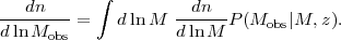 |
(150) |
For a power-law mass function dn / dlnM = A M-α = Aexp(-α lnM) and log-normal scatter of variance σ2 = < (lnMobs - lnM)2 >, one can readily compute the observed abundance by completing the square, finding
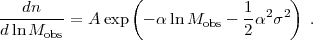 |
(151) |
From equation (151) it is evident that a shift in mass ΔlnM is degenerate with a shift in the variance Δσ2 = 2α-1 ΔlnM. (For a more rigorous argument that arrives at the same conclusion, see Lima and Hu 2005.) Thus, if the mass scale is controlled with an accuracy ΔlnM, then the scatter must be controlled with an accuracy Δσ2 = 2α-1 ΔlnM. If we further set Δσ2 = 2σΔσ, we arrive at Δσ = α-1 σ-1 ΔlnM. The fractional accuracy with which σ must be known to avoid competing with ΔlnM scales as σ-2, so the requirement is much less demanding if the scatter is smaller to begin with. As an illustrative example, we set α = 3 and σ = 0.2, which is roughly appropriate for SZ and likely slightly optimistic for optical. We find that the uncertainty due to errors in the scatter becomes comparable to that from errors in the mass when Δσ ≈ 1.7ΔlnM. For Stage III experiments with weak lensing calibration, yielding ΔlnM ≈ 2%, the scatter needs to be known at the Δσ ≈ 0.04 level, a value in agreement with the more rigorous estimate by Rozo et al. (2011b) and likely to be achievable in the near future (see, e.g., Rykoff et al. 2012). If Stage IV experiments reach 0.5% precision, the corresponding uncertainty in the scatter must be below 0.01 (absolute, not fractional), which is difficult to achieve from an ab initio calculation but may be possible with statistical calibration methods.
Finally, we must consider the possibility that, in addition to extended tails reflecting contamination and incompleteness, the core of P(X|M, z) deviates from log-normal form. This problem was considered by Shaw et al. (2008), whose discussion we paraphrase here. An observable-mass relation can be approximated by
 |
(152) |
known as the Edgeworth expansion. Here G is a Gaussian of zero mean and unit standard deviation, x = (lnX - <lnX >) / [Var(lnX | M, z)]1/2, γ is the skewness of the distribution, and κ is the kurtosis. For a power-law mass function dn / dlnM ∝ M-α, it is straightforward to check that the resulting cluster abundance is
 |
(153) |
where (dn / dX)0 is the abundance for a purely log-normal distribution. (Note that this α is also the logarithmic slope of the cumulative halo mass function dlnN / dlnM that appears in our earlier discussion.)
Setting α = 3 and assuming 10% scatter for X-ray masses, a 3% correction to the abundance — equivalent to a 1% correction in the mass — requires extreme non-Gaussianity with γ ≈ 7 or κ ≈ 90. Numerical simulations, on the other hand, predict distributions of X-ray observables that are close to log-normal (see, e.g., Stanek et al. 2010, Fig. 8; Fabjan et al. 2011, Fig. 3). We therefore do not expect X-ray studies to be sensitive to departures from a log-normal P(X|M, z). For [Var(lnX | M, z)]1/2 = 0.2, typical for SZ and perhaps achievable for optical, a 3% abundance change arises from γ ≈ 0.8 or κ ≈ 6, still quite large deviations from Gaussianity. For [Var(lnX | M, z)]1/2 = 0.4 these numbers drop to 0.1 and 0.35, respectively, so with this level of scatter a moderate degree of non-Gaussianity can have noticeable impact on the predicted abundances. For example, a Poisson distribution for a cluster with <N> = 10 galaxies corresponds to a skewness γ ≈ 0.3. This discussion demonstrates the value of finding improved optical richness estimators that have lower scatter relative to mass (Rozo et al. 2009, Rykoff et al. 2012).
Figure 29 shows the impact that various elements of P(X|M, z) can have on the recovered cluster counts. For illustrative purposes, we assume that X is an observed mass and show the change in the observed mass function due to changes in P(Mobs|M, z). For our reference model, we assume Mobs is unbiased and has log-normal scatter σ = 0.2, and we compute the cumulative cluster counts above Mobs for our fiducial cosmology at z = 0.6 in a redshift bin of width Δz = 0.1. Results at other redshifts are qualitatively similar.
 |
Figure 29. Relative change in cluster abundances at z = 0.6 as a function of mass due to a 2% bias in the mass (ΔlnM = 0.02), raising the log-normal scatter σ from 0.2 to 0.25, or introducing skewness γ = 1 in P(X|M, z) (solid, dashed, and dot-dashed curves, respectively). The statistical error in number counts for A = 104 deg2 is shown by the dotted line. The sensitivity of ΔlnN to systematic errors in the mass, scatter, or skewness can be estimated using the rule-of-thumb approximations in equations (154)-(156). |
Solid, dashed, and dot-dashed curves show the change in the cumulative number counts ΔlnN if Mobs is biased by 2% (ΔlnM = 0.02), if the scatter is increased from σ = 0.2 to σ = 0.25, or if the skewness is increased from γ=0 to γ=1 using the Edgeworth expansion. For reference, we also show the statistical error on the cluster counts for A = 104 deg2 as a dotted line. The details of P(X|M, z) affect the recovered cluster counts, and the impact is larger at higher masses than at lower masses. Moreover, the relative impact of skewness to scatter and of scatter to bias is mass dependent, with lower masses being more robust to uncertainties in the scatter and skewness. This is as expected: the shallower the slope of the mass function, the less important the details of P(X|M, z). The systematic offsets in Figure 29 are well approximated (to ≈ 10% and 30% for scatter and skewness respectively) by the rule-of-thumb calculations we have described above, specifically
 |
(154) (155) (156) |
Given the values of ΔlnN and α expected for a survey (Fig. 26; typical values ΔlnN ≈ N-1/2 and α ≈ 3), one can use equations (154)-(156) to infer the uncertainties ΔlnM, Δσ, and Δγ required to keep a cosmological analysis limited by abundance statistics.
6.4.4. Theoretical Systematics
Predicting observed cluster counts via equation (149) requires knowledge of the halo mass function dn / dM for any cosmological model under consideration. If the fractional uncertainty in dn / dM exceeds the observational error in cluster counts ΔlnN, or if the equivalent mass scale uncertainty exceeds the mass calibration error ΔlnM, then cosmological constraints will be limited by theoretical uncertainty rather than by observational errors. The study of Tinker et al. (2008) finds agreement in dn / dM at the ≲ 5% level among multiple simulations by different groups for a ΛCDM cosmological model with WMAP3 parameters. This is roughly the level required for large area surveys of M > 4 × 10¹⁴ M⊙ clusters in Δz = 0.1 bins, though higher accuracy is needed for lower mass thresholds (for detailed discussion see Cunha and Evrard 2010, 2010Wu et al. ). The formula (39) describes Tinker et al.'s z = 0 results accurately, but at redshifts z = 0.5-2.5 they find deviations of ~ 10-30% from this "universal" prescription. While these deviations are themselves numerically calibrated, their existence suggests that the mass function may depend on the dark energy model even when expressed in terms of the σ(M) relation as in equation (39). In addition, consistency in halo definitions is clearly critical. For instance, Bhattacharya et al. (2011) find that mass functions in their suite of wCDM simulations — which are calculated using friends-of-friends halo finders — deviate by up to 10% from a fitting formula calibrated on their ΛCDM simulation suite. It seems likely that Stage III and certainly Stage IV experiments will need to move to emulator based methods with comprehensive N-body libraries (e.g., Lawrence et al. 2010) rather than simple fitting formulae.
While further N-body work is needed to interpret future surveys,
dark matter evolution is straightforward in principle,
and the problem should yield to sufficient applications of
computational force. Baryonic evolution is potentially
a thornier issue. Some X-ray studies suggest a depletion of baryonic mass
(stars + hot gas) relative to the universal
Ωb /
Ωm
ratio by 20-30% within the Δ = 500ρc radius,
with systematically larger depletion in less massive clusters (e.g.,
Giodini et
al. 2009).
For Ωb /
Ωm = 0.17,
a 20% deviation in baryonic mass is a 3.4% deviation in total
mass, and thus comparable to or larger than the statistical mass
calibration errors achievable with stacked weak lensing
(Figure 28), as well as the precision required to
achieve the statistical limits of large cluster surveys
(Figure 23d).
Hydrodynamic simulations can explain baryon depletions
comparable to those observed
(Young et
al. 2011),
but the magnitude and even the sign of the baryonic effects depend on
the star formation and feedback physics (e.g.,
Stanek et
al. 2009,
Cui et al. 2012).
Furthermore, because the baryons influence the dark matter profile, they
can have substantial impact (~ 15%) on the total mass
within a high overdensity threshold (e.g., the
Δ = 500ρcrit
threshold frequently adopted in X-ray analyses; see
Stanek et
al. 2009).
In all of these simulations the corrections are smaller at larger radii,
so defining halo boundaries at lower overdensity
(such as the Δ = 200
 convention used here) is beneficial in this respect.
It may be possible to calibrate baryonic effects well enough with simulations and detailed observations of selected systems to remove them as a source of systematic uncertainty, but this problem will require concerted effort, particularly when Stage IV experiments get underway. By the same token, if stacked weak lensing is the primary mass calibration tool, then one must also develop robust theoretical models for predicting the weak gravitational lensing signal, which in turn requires that the halo-mass correlation function be characterized at the same level as ΔlnM. Current analytical models are accurate only at the ≈ 10%-20% level (Hayashi and White 2008), so this is another area that requires further theoretical study.
A final caveat related to the halo mass function is that primordial non-Gaussianity could alter its form (e.g., Weinberg and Cole 1992, Dalal et al. 2008, Grossi et al. 2009, LoVerde and Smith 2011, D'Amico et al. 2011) and thereby change the cluster abundances predicted for a given dark energy model (e.g., Cunha et al. 2010, Pillepich et al. 2012). Of course, evidence for non-Gaussian initial conditions would be exciting in its own right, with important implications for early-universe physics. However, it appears that the levels of non-Gaussianity that would have significant impact on cluster abundances are already ruled out by other constraints, unless one allows the magnitude of the non-Gaussianity to be scale-dependent (e.g., Hoyle et al. 2011, Paranjape et al. 2011). Given the strong theoretical prior for Gaussian initial conditions and the multiple observational probes that could detect and characterize primordial non-Gaussianity if it exists, we think it unlikely that non-Gaussianity will limit the power of cluster abundances as a probe of dark energy and modified gravity.
As discussed in Section 6.2, X-ray observations, possible only from space, have played a central role in nearly all cluster cosmological studies to date. The ROSAT All-Sky Survey has been the basis for many of the cluster samples used in these studies (Table 4). Pointed observations with a variety of telescopes, especially XMM-Newton and Chandra, have been the basis of mass calibration for X-ray observables and the source of most empirical knowledge about the physics of the intracluster gas. Ongoing XMM-Newton surveys will expand the dynamic range and size of X-ray catalogs over the next few years. The most important advance will come with the eROSITA mission (Merloni et al. 2012), which should produce the definitive all-sky survey of massive (M ≳ 4 × 10¹⁴ M⊙) clusters out to z ≈ 1, with an extended tail of higher redshift clusters reaching z ≈ 2. Follow-up X-ray studies at higher angular resolution will help better assess point-source contamination and will improve the mass calibration of the eROSITA catalog. For comparable numbers of clusters, X-ray catalogs offer significant advantages over SZ or optical catalogs because of the low scatter expected between X-ray observables and halo mass, which reduces sensitivity to uncertainties in the width and form of the observable-mass relation (Section 6.4.3).
For SZ searches, ground-based telescopes have higher sensitivity than space observatories because of their larger collecting area and higher angular resolution. The larger beam size of the Planck observatory (≈ 5 arcmin) relative to SPT and ACT (≈ 1 arcmin) reduces its ability to detect high redshift systems. Nonetheless, the all-sky nature of Planck observations is an important asset, and the Planck catalog of high mass clusters will be useful both for direct cosmological constraints and for cross-correlation studies with clusters identified at other wavelengths. Thus, we view the Planck, SPT, and ACT surveys as highly complementary. Any future CMB space mission designed to probe inflation physics and primordial gravity waves would also produce a much more sensitive all-sky SZ cluster catalog, provided it achieved high angular resolution.
Turning to optical searches, space observatories provide little advantage for cluster detection at z ≲ 1, since cluster detection does not gain much from the improved image resolution achievable from space. However, as discussed in Section 6.3.2, space-based near-IR imaging is highly desirable for extending (rest-frame) optical cluster catalogs to z ≈ 2. In the near future, such searches will rely on Spitzer data, as in the case of ISCS (Eisenhardt et al. 2008), SpARCS (Wilson et al. 2006), and the recently approved 100 deg2 Spitzer-SPT Deep Field. Additional IR data is or will soon be available from surveys like VHS, UKIDSS, and WISE, which may allow for high redshift cluster finding (Gettings et al. 2012). The VIKING survey, covering ≈ 1500 deg2, should be sufficiently deep to allow for robust cluster detection at z > 1. In the longer term, IR imaging from Euclid and/or WFIRST could make a key contribution to high redshift cluster surveys. High redshift cluster detection should also be feasible with extremely deep optical imaging from the ground, like that planned for LSST, which should reach z ≈ 1.5.
In the long run, however, the most important contribution of space
observations to cluster cosmology will come via weak lensing mass
calibration rather than cluster finding. The statistical error of WL
mass calibration scales as
g-1/2, where
g is
the source surface density. As can be seen from
Figure 28,
a surface density
g ≈ 30
arcmin-2 is
required to reduce mass calibration error below the statistical
abundance error, and even then only for z ≲ 0.5.
This source density is expected for an optical space mission
like Euclid, but it is probably higher than can be achieved
by ground-based observations, even with the depth and image
quality of LSST. The cluster counting error and
mass calibration error both scale with survey area as
A-1/2,
so the area effect cancels out if the cluster and WL surveys
overlap completely. If the cluster survey covers a larger area (e.g.,
the all-sky eROSITA catalog), then the WL source density required
to saturate the halo statistics limit is even higher.
Reaching the calibration accuracy allowed by the source galaxy
statistics also requires excellent control of shape measurement
systematics, generally expected to be lower from a
space-based platform, and photo-z systematics, which probably
require space-based IR imaging to achieve the stringent demands implied
by Figure 28.
More generally, if the error in WL mass calibration sets the
ultimate limit of cluster measurements of fluctuation growth,
as we have speculated it will, then the achievable error
on σ11,abs(z) scales as
g-1/2, or as
(Δγ)sys-1 if the WL measurements
are themselves limited by a shear measurement
systematic
(Δγ)sys.
We expect cluster abundance studies to undergo substantial and steady improvements over the next decade and beyond. In the near term (≲ 3 years), we anticipate advances in X-ray, SZ, and optical cluster studies. The XMM Cluster Survey (XCS) and XMM XXL Survey will yield much larger X-ray cluster samples at z ≳ 0.3. Planck will produce the definitive all-sky SZ catalog of massive clusters out to z ≲ 0.7, while SPT and ACT will probe z ≳ 0.7 cluster populations over thousands of square degrees for the first time. In the optical, continuing studies with the SDSS will lead to improved cluster finders and richness estimators, as well as improved weak lensing calibration thanks to better centering and better source photometric redshifts. On a comparable time scale, the RCS-2 survey will obtain g, r, and z imaging to a nominal depth of r ≈ 24.8 (roughly 2 magnitudes deeper than SDSS) over 1000 deg2, yielding the first large area optical cluster catalog extending to z ≈ 1. Relative to the results shown in Figure 22, these X-ray, SZ, and optical studies will improve the low redshift σ8 - Ωm constraint and extend it, at somewhat lower precision, to z ≈ 0.5-1. At the same time, improved calibration and cross-checks among surveys will test for and reduce remaining sources of systematic error.
In the medium term (≈ 3-8 years), several new optical surveys will cover thousands of deg2 with greater depth than SDSS and larger area and/or more photometric bands than RCS-2. These include the Kilo-Degree Survey (KIDS, 1500 deg2 in ugriz), DES (5000 deg2 in grizY), PS1 (15,000 deg2 in grizY), and the Hyper-Suprime Camera survey (HSC, 1500 deg2 in grizY). These surveys should significantly improve the cosmological constraints relative to RCS-2, thanks to higher cluster numbers, lower statistical errors in weak lensing mass calibration, and better control of photometric redshift uncertainties. The VIKING survey will cover 1500 deg2 at near-IR wavelengths (ZYJHKs) at sufficient depth to allow cluster identification and accurate photometric redshifts at z = 1-2. In addition, all of these surveys will overlap with Planck, and often with either the ACT or SPT surveys, which can further enhance the utility of both sets of catalogs. DES in particular is designed to cover the entire footprint of the SPT SZ survey.
With launch expected 2013-2014, eROSITA will produce the ultimate all-sky catalog of massive clusters (see Section 6.5). The optical imaging surveys will allow weak lensing calibration of the eROSITA mass-observable relations, with multiple independent surveys affording larger overlap area and thus more precise calibration. This combination of X-ray selection and optical WL calibration offers bright prospects for the coming decade of cluster cosmology. Optical surveys will further extend this leverage by probing cluster abundances to masses below those probed by eROSITA.
On a longer timescale, LSST plans to image 20,000 deg2 of high-latitude sky in six bands (ugrizY), with each single pass comparable in depth to the medium-term surveys described above and co-added data reaching 2.5-3 magnitudes deeper. The increased depth of LSST should allow one to cleanly select galaxy clusters out to z ≈ 1.5. While the greater dynamic range of the cluster catalogs will be an asset in itself, LSST's most important contribution to cluster cosmology will be in the form of improved WL mass calibration, both for eROSITA and for LSST's own clusters. Euclid could provide even better WL calibration over a similar sky area, while WFIRST should achieve a high WL source density but over a smaller survey area. The IR sensitivity of Euclid and/or WFIRST should also enable cluster searches at z ≈ 2 and beyond.
We have argued throughout this section that mass calibration will be the likely limiting factor in cluster studies of cosmic acceleration, and that stacked weak lensing is the most promising avenue to achieve accurate mass calibration. Figure 30 combines information from Figures 24 and 28, showing the fractional error on σ11,abs(z) in Δz = 0.1 bins that can be achieved with a 104 deg2 cluster survey, using the WL mass calibration errors we have forecast for Stage III (left panel) or Stage IV (right panel) source densities. With Stage III lensing calibration, errors on σ11,abs(z) are below 1% at z ≈ 0.5 for cluster mass thresholds of 1-2 × 10¹⁴ M⊙, and ~ 1.5% for a mass threshold of 4 × 10¹⁴ M⊙. With Stage IV lensing calibration, the peak sensitivity is better than 0.5% for the lower mass thresholds and better than 1% for the 4 × 10¹⁴ M⊙ threshold.
 |
Figure 30. Error on σ11,abs(z) achievable by measuring cluster abundances in a redshift bin z = zc ± 0.05 in a 104 deg2, assuming mass calibration via stacked weak lensing with Stage III or Stage IV source densities. We assume that all geometric cosmological parameters — most significantly the comoving volume element and the matter density parameter Ωm — are held fixed, being effectively constrained by a joint CMB+SN+BAO+WL experiment. Also shown for comparison are the forecast constraints on σ11,abs(z) derived from such a joint analysis using our fiducial Stage III and Stage IV surveys, assuming a w0 - wa parameterization of dark energy and allowing deviations from GR parameterized by G9 and Δγ (see Section 8.4 for details). |
The additional red and blue curves in Figure 30 show the forecast constraints on σ11,abs(z) for a fiducial Stage III (blue) or Stage IV (red) program combining SN, BAO, WL, and CMB data as discussed in Section 8. These forecasts assume a w0 - wa dark energy model and allow departures from GR-predicted growth described by an overall multiplicative offset G9 and a growth index deviation Δγ (see Section 2.2). The fiducial programs are defined in Section 8.1. If WL systematics are controlled at the level assumed in these fiducial programs then they should be negligible for cluster mass calibration relative to statistical errors, so we have not included them in computing ΔlnM.
From Figure 30 we see that a 104 deg2 cluster survey with Stage III WL calibration data can easily exceed the σ11,abs(z) precision expected from the Stage III CMB+SN+BAO+WL program, by as much as a factor of ≈ 3 for a threshold of 1014 M⊙. Similarly, cluster constraints with Stage IV WL calibration improve on the fiducial Stage IV σ11,abs(z) precision without clusters by a factor of ≈ 2. The visual impression that clusters can outperform the fiducial program only at z ≈ 0.4-0.8 but perform worse at high and low redshifts is artificial, since the CMB+SN+BAO+WL curves assume a smooth growth model while the cluster constraints in Figure 30 are those that can be achieved from galaxy clusters within each individual redshift bin. For Figure 30 we have assumed that errors on Ωm and dVc(z) are negligible. While the assumption for dVc(z) should prove reasonably accurate, the forecast CMB+SN+BAO+WL errors on Ωm (4% and 1% for Stage III and Stage IV, respectively) are larger than our assumed WL mass calibration errors for M ≲ 2 × 10¹⁴ M⊙ (see Figure 28). In practice, therefore, the fractional errors in Figure 30 would apply not to σ11,abs(z) but to the parameter combination σ11,abs(z) Ωmq, with q ≈ 0.4. We return to these points in Section 8.4 below, where we discuss the improvements in constraints on the dark energy equation of state and on G9 and Δγ achievable with clusters.
If some alternative mass calibration method proves better than stacked weak lensing, then the situation could be even better than Figure 30 suggests. This would be especially true for Stage III, where the WL source density is the clear limiting factor on the overall error. For our assumed Stage IV source density, the uncertainty from WL mass calibration is already close to the statistical uncertainty in cluster counts at z ≲ 0.6. Conversely, the situation would be worse than Figure 30 suggests if some other systematic uncertainty — e.g., contamination, miscentering, theory, or WL photo-z calibration — makes it impossible to achieve the statistical limits of the WL mass calibration.
In summary, our analysis indicates that cluster abundances with masses calibrated by stacked weak lensing could provide strong tests of cosmic acceleration models, beyond those afforded by the 2-point WL statistics described in Section 5. However, achieving this potential requires that mass calibration uncertainties be controlled at the 1-3% level for Stage III and at the 0.5-1.5% level for Stage IV. We see no obvious show stoppers, but the challenge is a demanding one.
66 Analogous to mass-to-light ratio, but with galaxy number instead of integrated luminosity. Back.
67 For example, in our fiducial cosmology at z = 0.6, the matter variance in a volume of Δz = 0.1 and area 10,000 deg2 is σ(V) ≈ 0.2%, and the mean halo bias is ≈ 3.0 and ≈ 5.7 for mass thresholds of 1014 M⊙ and 4 × 10¹⁴ M⊙, respectively. Back.
68 The distinction between statistical calibration via stacked weak lensing and direct calibration using weak lensing mass measurements is not a sharp one, and both methods share the virtue that the relation between mass and weak lensing signal is governed by well understood gravitational physics. By "stacked weak lensing" we mean to emphasize the case where (a) the WL measurements come from a large area imaging survey that overlaps the cluster catalog (and may have been used to create it) rather than from cluster-by-cluster follow-up observations, and (b) the S/N of the mass measurement for any individual cluster may be ≤ 1, though the S/N for the ensemble is high. Back.