5. WEAK LENSING

The subtle distortion of shapes of distant galaxies by gravitational lensing is a powerful probe of both the mass distribution and the global geometry of the universe. It has, however, turned out to be one of the most technically difficult of the cosmological probes. This section will cover the range of applications of weak lensing (which we will sometimes abbreviate to WL), the recent and planned weak lensing surveys, and the technical aspects of weak lensing image processing and control of systematics. By covering the latter subjects in some detail (including some methods that we think have been under-appreciated or under-utilized), we hope to stimulate further progress and be helpful to readers who are already experts in weak lensing.

This section is organized as follows: we begin with a qualitative overview of weak lensing and its uses (Section 5.1). We then go into a mathematical treatment of the various statistics that can be used and their dependences on the background cosmology and matter power spectrum (Section 5.2). We then review the observational results from recent weak lensing surveys (Section 5.3). Section 5.4.1 discusses the statistical errors and cosmological sensitivity of cosmic shear surveys at a rule-of-thumb level; we expect this to be a useful entry point for readers interested in understanding survey design. We then turn to more technical aspects of survey design and analysis, including source redshift estimation and the galaxy populations of optical/near-IR and radio surveys (Sections 5.4.2-5.4.4), CMB lensing (Section 5.4.5), the measurement of galaxy shapes (Section 5.5), and astrophysical uncertainties (Section 5.6). We summarize the major systematic errors and mitigation strategies (Section 5.7). We finally consider the advantages of a space mission for weak lensing (Section 5.8) and prospects for the future (Section 5.9).

Some of the material in this section is technical and in a first reading may be either skipped or skimmed; but given that so much of the promise of weak lensing depends on these issues, we felt compelled to include them. The more technical sections have been denoted with an asterisk (*). They may be thought of as analogous to, e.g., the "Track 2" material in Misner et al. (1973).

5.1. General principles: Overview

The images of distant galaxies that we see are distorted by gravitational lensing by foreground structures. In rare cases, such as behind clusters, one observes strong lensing: the deflection of light by massive structures can result in multiple images of the same background galaxy. More often, however, images of galaxies are subjected only to weak lensing: a small distortion of their size and shape, typically of the order of 1%. Since one does not know the intrinsic size or shape of a given galaxy, weak lensing can only be measured statistically by examining the correlations of shapes in deep and wide sky surveys. However, the payoff if these statistical correlations can be measured is enormous: weak lensing provides a direct measure of the distribution of matter, independent of any assumptions about galaxy biasing. Since this distribution can be predicted theoretically, even in the quasilinear regime, and since its amplitude can be directly used to constrain cosmology (unlike for galaxy surveys where one must marginalize over the bias), weak lensing has great potential as a cosmological probe.

In principle, one may attempt to observe either the shearing of galaxies (shape distortion) or their magnification (size distortion). In practice, the shape distortions have been used much more widely, since the mean shape of galaxies is known (they are statistically round: as many galaxies are elongated on the x-axis as on the y-axis) and the scatter in their shapes is less than the scatter in their sizes.

A variety of statistical approaches have been used to extract information from weak lensing shear (see later subsections for references). The simplest is the angular shear correlation function, or its Fourier transform, the shear power spectrum. These are related to integrals over the matter power spectrum along the line of sight, and as such in the linear regime at low redshift they scale as ∝ Ω_m² σ₈². ²⁸ Since the angular power spectrum is rather featureless, more information can be extracted via tomography — the measurement of the shear correlation function as a function of the redshifts of the galaxies observed, including the use of cross-correlations between redshift slices. Information on the relation between galaxies and matter can be obtained via galaxy-galaxy lensing, i.e., the correlation of the density field of nearby galaxies with the lensing shear measured on more distant galaxies. In the linear regime, the galaxy-galaxy lensing signal scales as ∝ b Ω_m σ₈² and thus provides information on the bias of the lensing galaxies, while in the nonlinear regime it probes individual galaxy halos and hence places constraints on the halo occupation distribution (Section 2.3). Combination of this with the galaxy clustering signal (which scales as ∝ b² σ₈²) enables one to eliminate the bias and measure Ω_m σ₈. The scaling of the galaxy-galaxy lensing signal as a function of the source redshift, known as cosmography, depends purely on geometric factors and hence can be used to partially ²⁹ construct a distance-redshift relation. Finally, the low-redshift matter distribution is non-Gaussian, so higher-order statistics such as the bispectrum or 3-point shear correlation function carry additional information.

For all of the applications of weak lensing to cosmology, deep wide-field imaging is essential. One can see this from a simple order-of-magnitude estimate. For a scatter in galaxy shapes of σ_γ ~ 0.2, measuring a 1% shear with unit signal-to-noise ratio requires ~ 400 galaxies (0.2 / √400 ≈ 0.01). Measuring the amplitude of density perturbations to 1% accuracy requires that this be done over ~ 10⁴ patches of sky, giving a requirement of order 10⁷ galaxies, which for a density of 15 resolved galaxies per arcmin² amounts to surveying 200 deg² of sky. This is the scale of the largest current surveys such as CFHTLS; in practice the errors from these surveys are likely to be closer to several percent due to "factors of a few" that we have dropped here, and due to the inclusion of systematic errors. The eventual goal of the weak lensing community is one or more "Stage IV" surveys (such as LSST on the ground and Euclid and WFIRST in space) that would measure shapes of ~ 10⁹ galaxies and achieve an additional order of magnitude in precision. Such surveys will have to face the daunting task of reducing systematic errors by another order of magnitude.

There are unfortunately many sources of these systematic errors, and most of the effort of the weak lensing community has been devoted to defeating them. One is the measurement of galaxy shapes: while gravitational lensing by a large-scale density perturbation can coherently align the images of many galaxies, this can also arise from shaking of the telescope or optical aberrations. The accurate determination of the point-spread function (PSF) of the telescope (usually based on observations of stars) and removal of its effects is thus critical. This problem gets much worse if one tries to model galaxies with sizes similar to or smaller than the PSF. High-resolution, stable imaging can help with this problem, motivating placement of future instruments at the best ground-based sites or in space. The determination of redshifts for the large number of source galaxies is also a concern. It is not practical to obtain a robust spectroscopic redshift of every galaxy, and hence "photometric redshifts" — estimates of galaxies' redshifts based on their broadband colors — are used. These must be calibrated with well-known biases, scatters, and outlier distributions. Finally, there are astrophysical uncertainties: galaxies can suffer "intrinsic alignments" (non-random orientations), and the matter power spectrum may deviate from pure CDM simulations at small scales. Much of our discussion here will be focused on the methodologies that have been developed to suppress systematics at each stage of the observations and analysis.

5.2. Weak lensing principles: Mathematical discussion

We will now go into greater detail on the mathematical aspects of weak lensing, both the construction of the weak lensing field and the various statistics that one can extract from it. The modern theoretical formalism of weak lensing traces back largely to the papers of Blandford et al. (1991), Miralda-Escudi (1991), and Kaiser (1992), though one can find roots in the much earlier papers of Kristian and Sachs (1966) and Gunn (1967).

5.2.1. Deflection of light in cosmology

Gravitational lensing gives a mapping from the intrinsic, unlensed image of the sources of light on the sky — the source plane — to the actual observable sky — the image plane. Our ultimate goal is to extract information about the statistics and redshift dependence of this mapping and use it to constrain cosmological parameters. Our task here is thus two-fold. First, we must derive the mapping function that relates the source to the image plane. However, since we do not know the intrinsic appearance of the sources, we cannot directly infer the lens mapping from observations. Therefore, our second task will be to determine what properties of the lens map can be measured, and with what accuracy.

In a fully general context, the lens mapping can be obtained by taking an observer and following the geodesics corresponding to that observer's past light cone. We will make some simplifying approximations here, namely that: (i) the spacetime is described by a Friedmann-Robertson-Walker metric with scalar perturbations and negligible anisotropic stresses (appropriate for nonrelativistic matter, scalar fields, and Λ); (ii) deflection angles are sufficiently small that we may use the flat-sky approximation; (iii) the evolution of perturbations is slow enough that we may neglect time derivatives of the gravitational potential Φ in comparison to spatial derivatives (i.e., nonrelativistic motion); and (iv) such perturbations are small enough that we may compute the lens mapping only to first order in perturbation theory. ³⁰ Within these approximations, we may write the angular coordinates (θ₁, θ₂) of a light ray projected back to comoving distance D_c (see eq. 7) in terms of the position (θ₁^I, θ₂^I) in the image plane as ³¹

(57)

where is the Green's function,

(58)

Here cot_k(D_c) is the cotangentlike function,

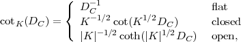(59)

with the dimensional curvature K defined in equation (8), and Φ is the Newtonian gravitational potential.

The potential derivative in equation (57) is evaluated at the position of the deflected ray θ_i(D_C1), so it represents an implicit solution to the light deflection problem. However, in linear perturbation theory (see our assumption iv above), we may evaluate it at the position of the undeflected ray. This is known as the Born approximation. When we do this, it is permissible to pull the angular derivative out of the integral and write

(60)

where ψ is the lensing potential:

(61)

Here it is important to remember that D_c represents the distance to the sources; one integrates over lens distances D_C1.

Equation (60) provides the mapping from the observed image plane to the source plane, θ_i^S(θ_i^I). In what follows, we will assume that this mapping is one-to-one: this is known as the regime of weak lensing. In the small portion of sky covered by very massive objects, the alternate regime of strong lensing occurs, in which several points in the image plane map to the same point in the source plane. Strong lensing is an important probe of the matter distribution in clusters, but we will not pursue it in this article; we briefly discuss some applications of strong lensing to cosmic acceleration in Section 7.10.

5.2.2. Cosmic shear, magnification, and flexion

We have now accomplished our first task: deriving the lens mapping from the matter distribution. However, we now need a way to classify the observables in the lens mapping. The potential ψ is of course not observable itself: like the Newtonian gravitational potential, its zero-level is arbitrary. Its angular derivative ∂ψ / ∂θ_i is the deflection angle: the difference between the true position of a source θ_i^S and its apparent position θ_i^I. However, since sources (in practice, galaxies) can be at any position, we cannot measure the deflection angle either.

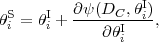
Let us now consider the second derivative of the lensing potential. It is simply the Jacobian of the mapping from image to source plane:

(62)

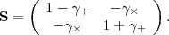
We have separated the 3 independent entries in the symmetric 2 × 2 matrix of partial derivatives into 3 components: the magnification (or convergence) κ and the 2 components of shear, γ₊ and γ_W. The magnification has three effects:

• It makes the angular size of a galaxy look larger by a factor of 1 + κ.
• It makes the galaxy appear brighter by a factor of the inverse-determinant of the Jacobian, 1 + 2κ, since lensing conserves surface brightness as dictated by Liouville's theorem.
• It dilutes the number density of galaxies by a factor of 1 - 2κ, since the angular spacing between neighboring galaxies is increased by a factor 1 + κ.

Magnification is a "scalar" in the sense that it is invariant under rotations of the (θ₁, θ₂) coordinate axes.

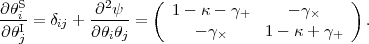
The shear stretches the galaxy along one axis and squeezes on the other: the image of an intrinsically round galaxy appears elongated along the θ₁ axis if γ₊ > 0 and along the θ₂ axis if γ₊ < 0. The γ_W component stretches and squeezes along the diagonal (45°) axes. The shear is a "spin-2 tensor" in the sense that under a counterclockwise rotation of the coordinate axes by angle δ, it transforms as

(63)

If all galaxies were round, then each galaxy would provide a direct estimate of the shear, since we could find the values of (γ₊, γ_W) that transformed an initially circular galaxy into the observed image. In reality, galaxies come in many shapes, and any such estimate of the shear components will have some standard deviation σ_γ known as the shape noise. But in an ensemble average sense galaxies are round — there are as many galaxies in the universe elongated along the θ₁ axis as the θ₂ axis. Thus, if we take N galaxies in the same region of sky, we may expect that the shear components in that region can be measured with a standard deviation of ~ σ_γ / √N. ³²

Several caveats are in order at this point, and they form the basis for most of the technical problems in weak lensing. One is that a circular galaxy re-mapped by the Jacobian (eq. 62) becomes an ellipse, but since in the real sky one does not observe a population of galaxies with homologous elliptical isophotes, there is no unique procedure to estimate the shear. Moreover, real telescopes, even in space, have finite resolution, and the observed image is convolved with a PSF that smears the galaxy and may introduce spurious elongation on some axis. These two problems together are referred to as the shape measurement problem. A more fundamental issue is that real galaxies are not randomly oriented: they have preferred directions of orientation that are correlated with each other and with large-scale structure, and thus contaminate statistical measures of the cosmic shear field. This is known as the intrinsic alignment problem. Finally, as already mentioned above, relating the lensing potential ψ to the gravitational potential Φ(z), and hence to cosmological parameters, requires accurate knowledge of the source galaxy redshift distribution, presenting the photometric redshift calibration problem. We will discuss all of these problems in Sections 5.4-5.7.

Measuring magnification κ has proven more difficult than measuring shear. One might imagine comparing the size, magnitude, or abundance of galaxies in some region of sky to a typical or "reference" value, but there is a very wide dispersion in galaxy sizes and magnitudes, and since some galaxies are too faint to observe even in deep surveys one cannot measure such a thing as the total number of galaxies. Rather, one can measure the cumulative number of galaxies brighter than some flux threshold, N(> F). If the number counts have a power-law slope α, i.e. N(> F) ∝ F^-α, then magnification will perturb this distribution by a factor

(64)

There are two competing effects here: in regions of higher magnification the galaxies appear brighter, which gives the 2ακ factor in equation (64), but there is also the dilution of galaxy number, which is responsible for the "-1" term. Unfortunately, for optical galaxies the observed number count slope is close to the critical value α≈ 1 for which magnification is not measurable. Moreover, the intrinsic clustering of galaxies gives large fluctuations in the number density that greatly exceed those due to lensing effects. For these reasons, magnification has lagged behind shear as a cosmological probe, and the cosmic magnification signal was not seen until Scranton et al. (2005) measured it using cross-correlation of foreground galaxies and background quasars. Minard et al. (2010) provide a more detailed analysis, using color information to simultaneously detect lensing magnification and reddening of quasars by dust correlated with intervening galaxies.

The most promising route to utilizing the cosmic magnification signal is to use scaling relations that relate the size of a galaxy (as quantified by, e.g., the half-light radius) to parameters that are magnification-independent and can be measured in photometric surveys (Bertin and Lombardi 2006), such as the surface brightness, the Sersic index, or (for AGN) variability amplitude. Huff and Graves (2011) present a first application of this "photometric magnification" method to galaxies, and Bauer et al. (2011) an application to quasars.

After shear and magnification comes the third derivative of the potential, i.e. the variation of shear and convergence across a galaxy. This effect is called the flexion, and it manifests itself via asymmetric banana and triangle-like distortions of an initially circular galaxy (Goldberg and Bacon 2005). Flexion has been measured by several groups (e.g. Leonard et al. 2007, Velander et al. 2011, Leonard et al. 2011), and there is a growing literature on the theory of flexion measurement that parallels the formalism required for shear measurement (e.g. Massey et al. 2007c, Schneider and Er 2008, Rowe et al. 2012). However, because of the extra derivative it is sensitive mainly to structure at the very smallest scales, so it is primarily a tool for cluster lensing rather than cosmological applications on larger scales.

5.2.3. Power spectra and correlation functions*

Just as for any other random field in cosmology, one may construct statistics for the cosmic shear field. The most popular are the power spectrum and its real-space equivalent, the correlation function.

To construct the power spectrum, we take the Fourier transform of the shear field,

(65)

When considering the shear produced by a plane wave perturbation of the lensing potential ψ(θ), it is convenient to rotate the Fourier-space components from the coordinate axis basis to a basis aligned with the direction of the wavevector, which is a preferred direction in the problem. The rotated components are called the E-mode and B-mode:

(66)

where tanϕ_l = l₂ / l₁, with l₁ and l₂ being the components of l in the pre-rotated coordinate system. Thus the E-mode of the shear field corresponds to galaxies that are stretched in the direction of the wave vector and squashed perpendicular to it, whereas the B-mode corresponds to stretching and squashing at 45° angles. One may then define the power spectra:

(67)

and similarly for C_EB(l) and C_BB(l). Rotational symmetry of structure in the universe guarantees that these depend only on the magnitude of l and not its direction, and reflection symmetry guarantees that C_EB(l) = 0.

In order to compute these power spectra, we need to express the Fourier modes in terms of those of the lensing potential. From the definition, equation (62), the shear is seen to be the derivative of the deflection angle and hence the second derivative of the lensing potential,

(68)

Using the replacement ∂ / ∂θ_i → il_i, we find in Fourier space

(69)

Substitution into equation (66) implies that

(70)

We thus arrive at the remarkable conclusion that cosmic shear possesses only an E-mode; the B-mode shear must vanish, and we have C_BB(l) = 0. Confirming this prediction of vanishing B-mode provides a valuable, though not foolproof, test for systematics in WL surveys.

The E-mode shear power spectrum is simply (l² / 2)² times the lensing potential power spectrum. The latter may be found from the Limber (small-angle) approximation ³³ in terms of the Newtonian potential power spectrum, yielding

(71)

(Here the power spectrum is evaluated at the redshift corresponding to D_C1.) We may put this in a more familiar form by recalling Poisson's equation, which tells us that the potential and matter density perturbations are related by

(72)

yielding

(73)

where the lensing window function ³⁴ is ³⁵

(74)

The window function describes the contributions to lensing of sources at D_c from lens structures at distance D_C1. Note that it vanishes as the lens approaches the source (D_C1 → D_c). In this equation, D_A1 is the comoving angular diameter distance (eq. 9) to D_C1: in a curved universe D_A1 ≠ D_C1. Note that in a flat universe, the window function reduces to

(75)

One may also define the angular correlation function of the shear for two galaxies separated by angle ϑ. Since the shear is a tensor, this is more complicated than the correlation function for scalars. Without loss of generality, we may rotate the coordinate system so that the galaxies are separated along the θ₁-axis, and then take the + and × components of the shear. We then define the shear correlation functions,

(76)

As in the scalar case, these are related to the power spectra:

(77)

where J₀ and J₄ are spherical Bessel functions. The expression for C_WW is similar, but with P_EE and P_BB switched. The correlation function {C₊₊(ϑ), C_WW(ϑ)}, if measured over all scales, contains exactly the same information as the power spectrum {C_EE(l), C_BB(l)}, as one can be derived from the other. Therefore, the choice of which to measure is usually a technical one based on the ease of data processing and handling of covariance matrices. The condition for no B-modes, C_BB(l) = 0 ∀ l, is more complicated in correlation-function space.

An infinite number of other second-order statistics (i.e., expectation values containing two powers of shear) can be constructed, such as the aperture-mass variance (Schneider et al. 1998), ring statistics (Schneider and Kilbinger 2007), and finite-interval orthogonal basis decompositions (a.k.a. COSEBIs, Schneider et al. 2010). These alternative statistics were introduced because they have useful properties from the point of view of data processing or systematics control — e.g., for separation of E and B modes, or restriction to a particular range of scales - but all of them are expressible as integrals over the power spectrum or correlation function.

Formulae such as (73) and (77) may be generalized to the full sky, as was first done for CMB polarization (Kamionkowski et al. 1997, Zaldarriaga and Seljak 1997), but for cosmic shear most applications involve small angular scales where the flat-sky approximation suffices. ³⁶

Having built the formalism to describe the statistics of weak lensing, we can now consider the proposed ways of using it to measure cosmology. Some methods will depend only on the expansion history of the universe, while others are sensitive to the growth of perturbations.

5.2.4. Method I: Cosmic Shear Power Spectrum*

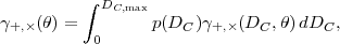
The conceptually simplest approach to using WL is to collect a sample of source galaxies, obtain an estimator for the shear at each galaxy, measure the correlation function or power spectrum, and do a comparison to equation (73). Of course not all galaxies are at the same redshift, but there is a probability distribution of distances p(D_c), and the observed mean shear in a particular region of sky is then

(78)

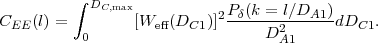
where D_C,max is the comoving distance to the farthest galaxy in the slice. The power spectrum of this field can then be written as

(79)

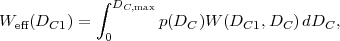
This is similar to equation (73) with W replaced by an effective window function,

(80)

which is simply the usual window function appropriately weighted over the source galaxies.

The cosmic shear power spectrum C_EE(l) is sensitive to many cosmological parameters. Being an integral over the matter power spectrum, it is ∝ σ₈² in the linear regime, although its behavior in the nonlinear regime is closer to ∝ σ₈³. It also contains two powers of Ω_m, so we expect that the most important dependences in the problem are that the WL power spectrum scales as ~ Ω_m² σ₈³. This is qualitatively correct, but the matter power spectrum and the mapping between D_A and D_c at finite redshift contain sensitivities to all of the cosmological parameters, and so a full answer to the question "what does the shear power spectrum constrain?" requires us to actually do the integral to obtain C_EE(l).

The sensitivity to every parameter is both a virtue of the WL power spectrum and its greatest fault: the featureless WL power spectrum contains too many parameter degeneracies. One way to break these degeneracies is to combine WL with other probes, as discussed in Section 8. However, there are also ways of using WL that provide additional information and break these degeneracies internally, as we now discuss.

5.2.5. Method II: Power Spectrum Tomography*

We can improve on the WL power spectrum constraints if we can split the source galaxies into redshift slices. In most practical cases, this would be done with photometric redshifts. In this case, instead of having a single power spectrum, we have N(N + 1) / 2 power spectra and cross-spectra; if we denote the slices by α, β ∈{1,2,...N}, then these spectra are

(81)

where W_eff,α is the effective window function for the α slice. Note that because the window functions are multiplied, this power spectrum depends only on the matter power spectrum at redshifts closer than that of the nearby slice, i.e. at z < min{z_α, z_β}. This makes sense because a given lens structure must be in front of both sources to contribute to the shear cross-correlation. Lensing analysis that splits samples by redshift and uses the redshift scalings to constrain cosmology is known as tomography.

Like the shear power spectrum, the tomographic spectra are sensitive to both the background geometry and the growth of structure: the shear power spectrum at l depends on the D_c(z) relation, on P_δ(k = l / D_A;z) as a function of redshift, and on the curvature K. ³⁷ With a single power spectrum C_EE(l) there is no hope of disentangling these functions with WL alone. One might hope that having the tomographic cross-spectra as a function of z_α and z_β would allow the relevant degeneracies to be broken. Unfortunately, such a program runs into three problems:

• A real WL survey has a maximum source redshift, and there is obviously no sensitivity to structures farther than this.
• There exist exact degeneracies among { D_c(z), P_δ(k = l / D_A;z), K} that lead to exactly the same lensing power spectra for all (l, z_α, z_β). The most obvious of these is the re-scaling degeneracy: since lensing measures only dimensionless shears, it cannot measure the absolute distance scale, only distance ratios. Two other degeneracies are discussed by Bernstein (2006); see also Section 5.2.7.
• The broad, smooth nature of the lensing window functions W_{eff, α}(D_c) implies near-degeneracies between power spectra at adjacent redshifts. For example, if one were to test a nonstandard cosmology in which P_δ(k, z) had a rapid oscillation in z superposed on the expected evolution, the rapid oscillation would contribute little to equation (81) and would be easily buried by statistical or systematic errors.

Despite these drawbacks, tomographic power spectra have far fewer parameter degeneracies than the shear power spectrum alone. More importantly, having N(N + 1) / 2 power spectra provides many additional opportunities for internal consistency tests and rejection of systematic errors.

Some examples of theoretical tomographic power spectra are shown in Fig. 16.

Figure 16. The E-mode shear power spectra predicted for the WMAP 7-year best fit cosmology (Ωm = 0.265, σ8 = 0.8, H0 = 71.9 km s-1 Mpc-1). The curves show power spectra for sources at z = 0.5 (bottom), 1.0, and 2.0 (top). The diagonal line shows the shot noise contribution at a source density of neff = 10 galaxies per arcmin2; for this power spectrum measurement the shot noise scales as neff-1. At small scales, where the noise power spectrum exceeds the signal, it is not possible to measure individual structures in the weak lensing map. However, with sufficient sky coverage, high-S/N measurement of the power spectrum or correlation function is still possible (see Section 5.4.1, particularly eq. 96).

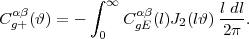
5.2.6. Method III: Galaxy-galaxy Lensing*

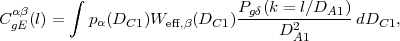
A third way to use weak lensing is to look not just at the shear power spectrum but at its correlation with the distribution of foreground galaxies. This subject is known as galaxy-galaxy lensing (GGL), and it is a powerful probe of the relation between dark matter and galaxies. The angular cross-power spectrum between the galaxies in one redshift slice α (the "foreground" or "lens" slice) and the E-mode shear in a more distant slice β (the "background" or "source" slice) is defined by

(82)

where δ_g^α is the 2-dimensional projected galaxy overdensity and δ_g^α is its Fourier transform, and α and β represent redshift slices. It can be computed via Limber's equation as

(83)

where P_{g δ}(k) is the 3-dimensional galaxy-matter cross-spectrum. The real-space correlation function of galaxy density and shear is

(84)

In the case where the foreground galaxy slice (α) is narrow - either due to use of spectroscopic foregrounds or high-quality photo-zs - the probability distribution in Limber's equation (eq. 83) becomes a δ-function, and the galaxy-matter cross-spectrum can be obtained.

One can also measure GGL by computing the mean tangential shear (i.e., shear in the direction orthogonal to the lens-source vector) of background galaxies around foreground galaxies as a function of radius. This view of the measurement is taken in many papers, but it is (almost) mathematically equivalent to correlating the shear field of the background galaxies with the density field of the foreground galaxies.

From the perspective of dark energy studies, the principal advantage of GGL over the shear power spectrum is observational: the shear is being correlated with galaxies rather than itself. A spurious source of shear, e.g. from imperfections in the PSF model, is a source of systematic error in the shear power spectrum, but in GGL it is only a source of noise because it is equally likely to arise in regions of high and low foreground galaxy density. The principal disadvantage of GGL is that its interpretation requires assumptions about the galaxies, which must ultimately be justified empirically.

Galaxy-galaxy lensing can be used in the linear, the weakly nonlinear, and the fully nonlinear regimes:

• Linear regime: In the linear regime, the galaxy-matter cross spectrum is P_{g δ}(k) = bP_δ(k), where b is the galaxy bias factor. Thus C_gE^αβ(l) is proportional to bσ₈², whereas the galaxy power spectrum is proportional to (bσ₈)². This provides a way to measure the linear bias of the galaxies and hence obtain σ₈. Unfortunately, one must reach very large scales (tens of Mpc) for linear perturbation theory to be valid at the few percent level of accuracy, and at these scales the signal-to-noise ratio of current GGL results is very low.
• Weakly nonlinear regime: At scales of order ~ 10h^-1 Mpc, nonlinear effects simply represent a correction to the linear theory, and one might hope that a judicious combination of observables can remove them. The key is to note that when stochasticity between galaxy and matter densities is included, the GGL signal is proportional to brσ₈², where r is the galaxy-matter cross-correlation coefficient, so all we require to extract b and σ₈ individually from GGL and galaxy clustering observables is a theoretical prediction for the stochasticity. This is a convenient result because simulations show that r = 1 is a much better approximation in the weakly nonlinear regime than b = constant. This type of analysis is also best done in real space rather than Fourier space so that the 1-halo contributions (see Section 2.3) to both clustering and lensing can be eliminated. A specific outline for how to do this, including the next-order perturbation theory corrections to r = 1 and comparison to simulations, is presented by Baldauf et al. 2010.
• Fully nonlinear regime: GGL can be used on the scale of individual halos (k ~ 1-10 Mpc^-1) to relate galaxy properties such as luminosity, color, and stellar mass to the properties of the host dark matter halo. Such relations cannot be predicted ab initio because of the complicated astrophysics involved. Empirical constraints on these relations are useful for dark energy studies mostly because they enable us to test some of the underlying assumptions of galaxy clustering models. To gain some cosmological power beyond the weakly non-linear regime, one can construct full galaxy HOD models and marginalize over their parameters, using both GGL and galaxy clustering as constraints (Yoo et al. 2006, Leauthaud et al. 2011, Leauthaud et al. 2012). Within the weakly non-linear regime, this approach effectively uses the HOD fits to compute the scale-dependence of br, drawing on the information in the small-scale galaxy clustering to improve the constraints.

Yoo and Seljak (2012) provide an extensive discussion of the cosmological constraints that can be derived from the combination of GGL and galaxy clustering, on small and large scales, in the simplified case where one isolates the population of central galaxies, so that there is one galaxy per dark matter halo.

Cluster-galaxy lensing is similar to GGL, but one takes clusters of galaxies rather than individual galaxies as the reference points (Mandelbaum et al. 2006, Sheldon et al. 2009). We will discuss this idea further in Section 6, arguing that it offers the most reliable route to calibrating cluster mass-observable relations and has the potential to sharpen cosmological parameter constraints significantly. Cluster-galaxy lensing may also be a useful tool for calibrating uncertainties in shear calibration and photometric redshifts, since the shear signal in the cluster regime is stronger and the cluster photometric redshifts themselves are usually well determined.

5.2.7. Method IV: Cosmography*

The previous sections motivate us to ask whether there is a way to combine the observational advantages of GGL with the model independence of the shear power spectrum. There is, although there is a large price to pay: one can only obtain geometrical information.

The idea is to consider narrow slices of galaxies centered at redshifts z_α < z_β < z_γ and measure the lensing of galaxies in slices z_β and z_γ by galaxies in the foreground slice z_α. The ratio of the galaxy-shear cross-spectra is, using equation (83),

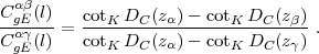(85)

One can see that all dependence on the power spectra and the distribution of galaxies has been cancelled, allowing a purely geometric test of cosmology. This is called the cosmography or shear-ratio test (Jain and Taylor 2003, Bernstein and Jain 2004).

One can see from equation (85) that cosmography can determine the cot_k D_c(z) relation up to any affine transformation, i.e. transformations of the form

(86)

which leave the ratios of differences of cot_k D_c(z)s unaffected. (Recall that cot_k D_c = 1 / D_c in a flat universe.) It is clear that a₁ is the familiar overall rescaling degeneracy: cosmography measures only dimensionless ratios and cannot distinguish two models with different H₀ butthe same values of Ω_m, w, etc. Precisely the same degeneracy afflicts the supernova D_L(z) relation because the absolute magnitude of a Type Ia supernova is not known a priori. The a₀ degeneracy is trickier, arising from the fact that ∞ is not a special distance in lensing problems. ³⁸ Finally, since only cot_k D_c(z) is measured, cosmography cannot by itself provide a model-independent measurement of the curvature of the universe. But aside from these three degeneracies — a₁, a₀, and K — the entire geometry of the universe over the range of redshifts observed is measurable.

Unfortunately, the aforementioned degeneracies are similar in functional form to the effects of Ω_m and w, and they have severely limited the application of cosmography thus far. This is particularly true for observations restricted to low redshift: if one Taylor expands the distance as tan_k D_c(z) = c₁ z + c₂ z² + c₃ z³ + ... then any cosmological model is degenerate with one that has (c₁, c₂) = (1, 0), and hence one must go through at least the z³ term before cosmography provides any useful information. For example, at (z_α, z_β, z_γ) = (0.25, 0.35, 0.70), the difference in the shear ratio (eq. 85) between an Ω_m = 0.3 flat ΛCDM cosmology and a pure CDM Ω_m = 1 cosmology is only 1%! In early work (Mandelbaum et al. 2005) cosmography was therefore used as a test for shear systematics rather than a cosmological probe.

The outlook for cosmography is much brighter as we probe to larger redshifts, or if we consider dark energy models with complicated redshift dependences that cannot be mimicked by the degeneracy of equation (86). A particularly promising possibility is to use cosmography with lensing of the anisotropies in the CMB (z = 1100) to obtain a much longer lever arm (Acquaviva et al. 2008). In principle one can also apply the cosmography method to strong gravitational lenses (see Section 7.10 below). Here the challenge is that different sources probe different locations in the lens, so one must be able to constrain the lens potential extremely well to extract useful cosmographic constraints.

5.2.8. Method V: Non-Gaussian Statistics*

The primordial density fluctuations in the universe were very nearly Gaussian, as evidenced by the CMB. In this case, the fluctuations are fully described by the power spectrum, and this has become the common language of CMB observations. However, nonlinear evolution makes the matter fluctuations and hence the lensing shear in the low-redshift universe highly non-Gaussian on small and intermediate scales. Therefore, many other statistical measures of the shear field have been proposed, the most popular of which is the bispectrum.

The bispectrum is obtained by taking the product of three Fourier modes:

(87)

Statistical homogeneity forces the three wave vectors involved to sum to zero so the bispectrum is actually a function of the triangle configuration; rotational and reflection symmetry then tell us that it depends only on the side lengths (l₁, l₂, l₃) ³⁹, which must satisfy the triangle inequality. Because there are 2 shear modes (E and B), there are actually 4 types of bispectrum: EEE, EEB, EBB, and BBB, but only EEE can be produced cosmologically. Limber's equation expresses it in terms of the 3-dimensional matter bispectrum,

(88)

The bispectrum contains information equivalent to the shear 3-point correlation function. The theory of transformations between the two and the implied symmetry properties have been extensively studied (Zaldarriaga and Scoccimarro 2003, Schneider and Lombardi 2003, Takada and Jain 2003, Schneider et al. 2005). Halo model based descriptions of the 3-point function are also available (e.g. Cooray and Hu 2001).

The original motivation to study the WL shear bispectrum was to break the degeneracy between Ω_m and σ₈ (e.g. Bernardeau et al. 1997, Hui 1999, Takada and Jain 2004). At low redshift, and on large scales where perturbation theory applies, the WL power spectrum is proportional to Ω_m² σ₈², whereas the bispectrum is proportional to Ω_m³ σ₈⁴; it contains three powers of the shear and hence three powers of Ω_m, but the matter bispectrum is generated by nonlinear interactions and is proportional to the square of the matter power spectrum, i.e., to σ₈⁴ rather than σ₈³. Unfortunately, this route to degeneracy breaking has proven difficult because of the low signal-to-noise ratio and high sampling variance of the bispectrum and because the degeneracy directions of the power spectrum and bispectrum are almost parallel in the (Ω_m, σ₈) plane. A more interesting application of the WL bispectrum in future surveys may be as a constraint on modified gravity theories, though this has not yet been well studied.

5.3. The Current State of Play

Weak lensing as a cosmological probe is only a decade old, although the ideas go back much further. Zwicky (1937) famously suggested gravitational lensing as a tool to determine cluster masses (although the discussion focused on strong lensing). We separately consider here the more recent history of cosmic shear studies, and of galaxy-galaxy lensing as a cosmological probe. Also the techniques and applications associated with lensing outside the optical bandpasses are sufficiently different that we place them in a separate section. Lensing by clusters is considered in the cluster section (Section 6).

5.3.1. Cosmic shear

Kristian (1967) described an initial attempt to measure statistical cosmic shear using photographic plates taken on the Palomar 5 m telescope. He even correctly identified intrinsic alignments as a systematic error, and noted that the distance dependence could be used to separate them from true cosmic shear. Interestingly, the objective of this analysis was to search for cosmological-scale gravitational waves or other large-scale anisotropies (Kristian and Sachs 1966). The author set a limit on the magnetic part of the Weyl tensor ⁴⁰ of ≲ 200 H₀^-2, which he describes as "about the best that can be done with this kind of measurement." Fortunately this has not remained the case - indeed it was improved upon by two orders of magnitude by Valdes et al. (1983).

The modern era of lensing studies was introduced by the availability of arrays of large-format CCDs. Mould et al. (1994) searched for cosmic shear and reached percent-level sensitivity, but did not detect a signal. Cosmic shear was finally detected in 2000 by several groups (Wittman et al. 2000, Bacon et al. 2000, Van Waerbeke et al. 2000), and in deeper but narrower data from HST (Rhodes et al. 2001, Refregier et al. 2002). Over the same period, several additional square degrees were observed with long exposure times in excellent seeing using ground-based telescopes (Van Waerbeke et al. 2001, Van Waerbeke et al. 2002, Bacon et al. 2003, Hamana et al. 2003). The first wide-shallow surveys were also carried out from the ground: the 53 deg² Red-Sequence Cluster Survey (Hoekstra et al. 2002) and the 75 deg² CTIO survey (Jarvis et al. 2003). These studies established the existence of cosmic shear, but at a level far below that which would be expected in Ω_m ~ 1 models normalized to the CMB. The large error bars in early studies meant that only a single amplitude could be measured, yielding a constraint on the combination σ₈(Ω_m / 0.3)^ν, where the exponent ν varied between 0.3 and 0.7 depending on the scale and depth. In the first detection of the cosmic shear bispectrum, achieved with the VIRMOS-DESCART survey, Pen et al. (2003) measured the skewness of the filtered shear signal and used it in combination with the power spectrum to rule out large-Ω_m, low-σ₈ solutions, finding Ω_m < 0.5 at 90% confidence. The deep COMBO-17 survey first detected the evolution of σ₈ as a function of cosmic time (Bacon et al. 2005).

However, the early studies of cosmic shear were not free of trouble. As one can see from Table 3, while most were broadly in agreement with σ₈ in the 0.7-0.9 range, a detailed comparison shows that the measurements were not all consistent. This discrepancy stimulated discussions about a number of possible ancillary issues with the data, such as the role of intrinsic alignments, whether the source redshift distribution N(z) was properly calibrated, and whether the models for the nonlinear power spectrum and assumptions about the P(k) shape parameter Γ could be leading to discrepancies. More seriously, most of the early measurements contained B-mode signals at levels not far below the E-mode. This was a clear signal of contamination of non-cosmological origin, probably PSF correction residuals. Also, intrinsic alignments of galaxies were detected at high significance even in the linear regime, at a level that represented a potentially serious systematic error even for then-ongoing surveys (Mandelbaum et al. 2006).

It was clear by 2006 that weak lensing was a very hard observational problem and that a great deal of work lay ahead to turn it into a precision cosmological probe. This resulted in a reduction in the rate of new cosmic shear results, the reorganization of the field into larger teams, and detailed looks at systematic errors ranging from optical distortions in telescopes to intrinsic galaxy alignments. Several wide-field optical surveys were ongoing at the time, including the deep 170 deg² CFHT Legacy Survey (for which cosmic shear was a key science driver) and the very deep multiwavelength COSMOS survey with high-resolution optical imaging from HST/ACS (Massey et al. 2007b, Schrabback et al. 2010). The CFHTLS presented some early results (Hoekstra et al. 2006, Semboloni et al. 2006a, Fu et al. 2008), but following this there was a rather bleak period of time. No new ground-based wide-field cosmic shear results were published, and no new large surveys were undertaken with HST, nor do future large HST weak lensing surveys seem likely. ⁴¹

In the past five years, however, great progress has been made in overcoming the difficulties that at first appeared so daunting. The community made a massive investment in algorithms to determine and correct for PSF ellipticities (we will review some of these in Section 5.5), and in investigating the physics that determines the PSF, including such complications as atmospheric turbulence (Heymans et al. 2012a). Equally important, these methods were tested in public challenges on simulated data (STEP1, Heymans et al. 2006; STEP2, Massey et al. 2007a; GREAT08, Bridle et al. 2010; GREAT10, Kitching et al. 2010; see further dicussion in Section 5.5). Progress was also made on astrophysical systematic errors. We learned that large-scale intrinsic galaxy alignments are strongest for luminous red galaxies (Hirata et al. 2007, Mandelbaum et al. 2011), and that the linear alignment model, once considered a crude analytical tool (Catelan et al. 2001), is in fact an excellent description of the observations of early-type galaxies at ≥ 10h^-1 Mpc scales (Blazek et al. 2011).

As a result of this great effort by the community, the Stage II weak lensing results are finally coming to fruition and yielding large data sets that pass the standard systematics tests (e.g., B-modes consistent with zero). Two groups (Lin et al. 2012, Huff et al. 2011 have performed a cosmic shear measurement using the Sloan Digital Sky Survey deep co-added region — a 120-degree long stripe observed many times over the course of three years as part of the SDSS-II supernova survey. These analyses used different methods to co-add their data and correct for the PSF ellipticity, and they imposed different selection cuts and hence had different redshift distributions, yet the results were in agreement (and slightly more than 1σ below the WMAP prediction for σ₈). The largest of the Stage II weak lensing programs was the CFHT Legacy Survey. After a thorough analysis, the lensing results and cosmological implications were recently published (Heymans et al. 2012b, Benjamin et al. 2012, Erben et al. 2012, Kilbinger et al. 2012, Miller et al. 2013). They appear consistent with the standard ΛCDM cosmology with WMAP-derived initial conditions, with the amplitude σ₈ measured to ± 0.03.

A summary of the current status of optical cosmic shear results is shown in Table 3.

5.3.2. Galaxy-galaxy lensing as a cosmological probe

Like cosmic shear, galaxy-galaxy lensing is an old idea. The earliest astrophysically interesting upper limit was that of Tyson et al. (1984), who used the images of 200,000 galaxies measured by the now-obsolete method of digitizing photographic plates to exclude extended isothermal halos with v_c > 200 km s^-1 around an apparent magnitude-limited sample of galaxies. Galaxy-galaxy lensing was observed at ~ 4σ by Brainerd et al. (1996), the first clear detection of cosmological weak lensing. Their analysis used a total of 3202 lens-source pairs in a field of area 0.025 deg². Several other detections followed this in deep surveys with limited sky coverage (Hudson et al. 1998, Smith et al. 2001, Hoekstra et al. 2003). However the full scientific exploitation of the galaxy-galaxy lensing signal — in contrast to cosmic shear — favors wide-shallow surveys over deep-narrow surveys, since the S/N in the shape-noise limited regime scales as only _source^1/2 rather than _source. Therefore, in the decade of the 2000s the leading galaxy-galaxy lensing surveys became the 92 deg² Red-Sequence Cluster Survey (RCS; Hoekstra et al. 2004, Hoekstra et al. 2005, Kleinheinrich et al. 2006) and eventually the 10⁴ deg² SDSS (references below). The availability of spectroscopic redshifts in the latter allowed the signal from low-redshift galaxies to be stacked in physical rather than angular coordinates, enabling the detection of features as a function of transverse separation. The spectroscopic survey also provided detailed environmental information, measures of star-formation history, and full 3-dimensional clustering data (e.g., correlation lengths and redshift-space distortions) for the lens galaxies.

The SDSS remains the premier galaxy-galaxy lensing survey today, for both galaxy evolution and cosmology applications, and it likely will remain so until DES and HSC results become available. The SDSS Early Data Release, comprising only a few percent of the overall survey, already detected the galaxy-galaxy lensing signal with high significance (Fischer et al. 2000, McKay et al. 2001). Some of the major results of cosmological importance from the SDSS galaxy-galaxy lensing program have been:

• The galaxy bias can be constrained directly by going to the very largest scales and measuring galaxy-galaxy lensing in the 2-halo regime. By dividing the galaxy clustering signal by the galaxy-mass correlation function, Sheldon et al. (2004) found for L_* galaxies a bias of b = (1.3 ± 0.2)(Ω_m / 0.27)r, where r is the stochasticity (presumably ~ 1 at the largest scales), with no evidence of scale dependence. ⁴², ⁴³

• The measurement of halo masses — or more accurately, HOD parameters (see Section 2.3) — with galaxy-galaxy lensing also enables one to predict the galaxy bias, by using the bias-mass relation b(M). One can in principle use this to constrain cosmological parameters, since the clustering of the lens galaxies can be measured and hence one can obtain σ_8,gal ≡ bσ₈. The results of this analysis on 300,000 lens galaxies at z ~ 0.1 were presented by Seljak et al. (2005). The direct constraints on σ₈ itself (with other parameters fixed) were uninteresting because the inferred bias at fixed halo mass is a decreasing function of σ₈, and the observable product σ₈b is almost independent of σ₈. However, cosmological parameters that change the shape of the power spectrum can be constrained quite well — e.g., a decrease in small-scale power can make halos rarer and hence decrease b without a compensating change in σ₈. This breaks degeneracies internal to the CMB alone. Combining with first-year WMAP data, Seljak et al. (2005) found that for the case of three degenerate neutrinos one must have Σm_ν < 0.54 eV (95%CL).
• The halo mass-concentration relation c(M) (e.g., Bullock et al. 2001) is not in and of itself especially useful as a dark energy probe; it depends somewhat on Ω_m, but also on baryonic physics. Nevertheless, testing it is important for any cosmological application of the 1-halo regime, including cosmic shear (King and Mead 2011), and galaxy-galaxy lensing is well suited to measuring it at a range of halo masses. (For clusters other techniques are available, such as strong lensing or X-ray measurements.) Mandelbaum et al. (2008) measured this relation across the 10¹² - 10¹⁵ M_⊙ range, finding c_200b(M) = (4.6 ± 0.7) M₁₄^{-0.13 ± 0.07}, where M is the halo mass in units of 10¹⁴ h^-1 M_⊙. The normalization is about 2σ below the theoretical predictions, but the discrepancy may well be a statistical accident, particularly given that other methods have led to larger concentrations.
• Reyes et al. (2010) tested GR by comparing the galaxy-mass correlation function, measured via weak lensing, to the galaxy-velocity correlation function, measured via redshift-space distortions. The SDSS luminous red galaxy sample was chosen due to its large volume. This measurement requires an overlapping spectroscopic and WL survey. They find that

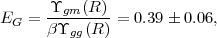  (89)

  where Υ is a filtered correlation function (averaged over scales R = 10 - 50 h^-1 Mpc) and β is the redshift-space distortion parameter of equation (43). The combination E_g is equal to Ω_m / f(z) at the redshift of the lenses, for which GR predicts Ω_m^0.45(z = 0.32) = 0.408 ± 0.029. This measurement establishes that the peculiar velocities of galaxies are, to ~ 15% precision, in agreement with expectations based on the potential structure traced by lensing.

All of these measurements will become possible with much smaller error bars once the Stage III WL experiments are operational. We look forward in particular to much smaller error bars on b / r and E_g derived from the largest scales, as well as improvements on c(M).

5.3.3. Lensing outside the optical bands

All wavelengths of light are gravitationally lensed. The optical ⁴⁴ is not special in this regard — rather, the emphasis on optical wavelengths has been technological, as this is the cheapest band in which to observe and resolve large numbers of galaxies at cosmological distances and obtain some redshift information. However, advances in technology in other wavebands have resulted in weak lensing being detected at several other wavelengths:

• In the radio, kilometer-scale interferometers are required to resolve extragalactic sources, and at the present time one cannot obtain a radio photo-z because of the featureless synchrotron spectra. However, Chang et al. (2004) detected cosmic shear of extended radio sources using the Very Large Array FIRST survey.
• Lensing of the CMB has been of interest for some time as it provides the most distant possible source screen. The first search was carried out in cross-correlation by Hirata et al. (2004) using luminous red galaxies in SDSS as the lenses and WMAP temperature anisotropies as the sources. The signal was detected three years later with combinations of SDSS and NVSS data, and two additional years of WMAP data (Smith et al. 2007, Hirata et al. 2008). Recently, the Atacama Cosmology Telescope (ACT) carried out a cosmic shear autocorrelation analysis using the CMB as a source and detected the signal at 4σ (Das et al. 2011). While apparently weak, this measurement shows that Ω_Λ > 0 using CMB data alone, without assuming a flat universe (Sherwin et al. 2011). The ACT and South Pole Telescope (SPT) collaborations are next planning polarization surveys, which should yield much higher S / N detections of lensing and provide constraints on the neutrino mass.

5.4. Observational Considerations and Survey Design

5.4.1. Statistical Errors

The forecasting of statistical errors on the cosmological parameters is much more involved for WL than for supernovae or BAO because of the complex dependence of the observables on the underlying model. Nevertheless, some intuition can be gained by making approximations to enable exact evaluation of the integrals. Specifically, we assume (i) a single source redshift z_s; (ii) a power-law matter power spectrum,

(90)

where the slope k^-1.3 is chosen to match that of the ΛCDM power spectrum at a scale of ~ 10 Mpc and the normalization is chosen to give the correct σ₈; (iii) evaluation of the normalization (1 + z)G(z) not at the true lens redshift z_l (over which we integrate from 0 to z_s) but at a "typical" lens redshift z_s / 2; and (iv) a flat universe. Then equation (73) gives

(91)

The variance per logarithmic range in l is

(92)

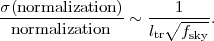
this is a measure of the shear variance at a particular angular scale θ~ l^-1. Recall that (1 + z)G(z) varies from ≈ 0.75 at z = 0 to one at high redshift (see Fig. 3). Since H₀ enters only in the combination H₀ D_c(z), and D_c(z) ∝ H₀^-1, we see again that the WL signal depend on relative rather than absolute distances.

In practice, equation (92) is only a rough guide because of deviations of P_δ(k) from a power law and the nonlinear enhancement of the matter power spectrum on small scales. Nevertheless, we can see several important features:

1. The typical shear, given by [Δ²(l)]^1/2, is of order 1% at cosmological distances (z_s ~ 1) and degree scales (l~ 100). The shear fluctuations are larger at smaller scales.
2. The shear power spectrum scales as ∝ σ₈². Assuming a known background cosmology and source redshift, a measurement of the power spectrum to X% determines σ₈ to an uncertainty of 1/2 X%. In the nonlinear regime the dependence of the shear power spectrum is closer to σ₈³, so in practice the constraint on σ₈ is better than equation (92) would suggest.
3. Alternatively, if one assumes perfect knowledge of the growth of structure (hence σ₈, Ω_m, and G), then the distance D_c(z_s) to the sources can be determined to an uncertainty of 1/2.3 X%. Lensing thus acts as a standard "ruler."
4. Measuring the shear power spectrum as a function of source redshift z_s allows one to measure some combination of the growth function and the distance as functions of redshift. However, one does not measure both separately. In order to simultaneously constrain the functional forms G(z) and D_c(z), lensing must be combined with another cosmological probe.
5. Systematic errors in any of the terms in equation (92) will bias the cosmology results. In particular, a 1% change in z_s, e.g. 1.00 → 1.01, changes the power spectrum by 2%. (This is the result of a full calculation, not evident by simple inspection of the equation.) Therefore, careful estimation of the source redshift distribution is required for a WL survey — a challenge when relying on photometric redshifts for the vast majority of sources.

The statistical uncertainty on the shear power spectrum is determined by two factors: sampling variance at low l and shape noise at high l. Sampling variance uncertainty is associated with the fact that there are only a finite number N of Fourier modes in the survey area, and consequently the fractional uncertainty in the power can be no smaller than √2/N (where the 2 arises because power is the variance of γ_l, not the rms amplitude). If we measure the power spectrum in a bin of width Δl, then the number of modes is N = 2lΔl f_sky, where f_sky is the fraction of the sky observed. This corresponds to a sampling variance uncertainty

(93)

If we measure modes up to some l_max, there are l_max² f_sky modes, and the sampling variance uncertainty in the normalization of the power spectrum is √2 f_sky^-1/2 l_max^-1.

At high l, the errors on the WL power spectrum become dominated not by the number of modes available but by how well each mode can be measured with a finite number of galaxies. Individual galaxies are not round, and so a shear estimator applied to a galaxy has an intrinsic scatter σ_γ ~ 0.2 rms in each component of shear (γ₊ or γ_W), for typical galaxy populations with rms ellipticity e_rms ~ 0.4 per component. This phenomenon is known as shape noise. Since it is uncorrelated between distinct galaxies (at least as a first approximation), shape noise produces a white noise (l-independent) power spectrum ⁴⁵,

(94)

where _eff is the effective number of galaxies per steradian (this is the true number of galaxies with a penalty applied for objects where the observational measurement error on the shear becomes comparable to σ_γ; see below). Since the cosmic shear C_EE(l) is decreasing with l, there is a transition scale l_tr where the shape noise becomes comparable to the lensing signal. Using equation (92), we estimate

(95)

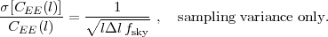
At angular scales smaller than θ ~ l_tr^-1, lensing cannot detect (at S/N > 1) a typical fluctuation in the density field. ⁴⁶ Statistical measurements are still possible, however, and the power spectrum can be measured to an accuracy of √2/N C_EE^shape(l) where N is the number of modes. Thus, in the shape-noise limited regime,

(96)

One can see from this equation that the fractional uncertainty on C_EE(l) in bins of width Δl / l ~ 1 increases with l for l > l_tr. Therefore we arrive at the important conclusion that the power spectrum is best measured at the transition scale l_tr: on larger scales sampling variance degrades the measurement even though individual structures are seen at high signal-to-noise ratio (SNR), and on smaller scales shape noise dominates. The aggregate uncertainty in the normalization of the power spectrum is thus of order

(97)

A full-sky experiment ⁴⁷ reaching tens of galaxies per arcmin² at redshifts of order unity would have l_tr ~ 1000 and so could measure the normalization of the power spectrum to a statistical precision of order 0.1%. This would be an unprecedented measurement of the strength of matter clustering. However, as we will see below, there are substantial statistical and systematic hurdles to such an experiment.

Finally, we consider galaxies measured at finite SNR. In the above analysis, we assumed that each galaxy provided an estimate of the shear with uncertainty σ_γ. At finite SNR there is also measurement noise σ_obs, so that each galaxy provides an estimate with error (σ_γ² + σ_obs²)^1/2. Using inverse-variance weighting, in the finite-SNR case the shape noise becomes equation (94), with the effective source density

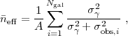(98)

where A is the survey area and the sum is over the galaxies. This is always less than = N_gal / A. The effective source density _eff is limited in part by the depth of the survey: σ_obs,i typically scales with integration time as ∝ t^-1/2, but once σ_obs,i ≪ σ_γ one no longer continues to gain. How long does this take? In Section 5.5.3, we will show that for nearly circular, Gaussian galaxies ⁴⁸

(99)

where r_psf and r_gal are the half-light radii of the PSF and the galaxy, respectively, and ν is the detection significance (in σs). Thus for galaxies with a similar size as the PSF, we expect to reach σ_obs = 0.1 (measurement noise half of shape noise) after integrating long enough to see the galaxy at 20σ.

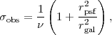
In principle, the summation in equation (98) is over all objects detected as extended sources, and any galaxy could be used if its detection significance is high enough. In practice, this is dangerous: while one might hope to obtain σ_obs = 0.1 on a galaxy with r_gal = 0.5r_psf and a 50σ detection, the "ellipticity measurement" on this galaxy consists of measuring the small deviation of the image from the PSF. Such a procedure tends to magnify systematic errors in the PSF model and is usually unadvisable. Therefore, most WL surveys impose a cutoff on r_gal / r_psf or some similar property.

5.4.2. The Galaxy Population for Optical Surveys

The design of a WL survey must begin by considering the population of galaxies. We will focus here on the population in the 3-dimensional space of redshift z, effective radius r_eff, and apparent AB magnitude in the I-band (a convenient choice for shape measurement with red-sensitive CCDs from the ground). The plots shown here are based on the mock catalog of Jouvel et al. (2009), which uses real galaxies from the COSMOS survey but fills in missing information for individual galaxies (e.g. redshifts or line fluxes) with photo-zs and models.

Figure 17 shows the mean surface density of galaxies and the median source redshift as a function of limiting magnitude I_ab for effective radius cuts of 0.15", 0.248", and 0.35". In general, one would like to use galaxies larger than the PSF to avoid amplification of systematics when applying a PSF correction to the shapes. The "effective radius" (EE50, for 50% encircled energy) of a typical ground-based PSF is ~ 0.35" under good conditions, corresponding to a FWHM of ~ 0.7". The 0.248" cut is a factor of √2 smaller, appropriate if one can make use of galaxies smaller than the PSF or has sufficient itendue to do the entire survey under the very best seeing conditions. Measuring galaxies at r_eff = 0.15" is well beyond present ground-based cosmic shear survey capabilities, for both algorithmic and PSF-determination reasons, and will likely require a space (or balloon) based platform.

Figure 17. The mean surface density of galaxies (top panel) and median redshift (bottom panel) as a function of limiting magnitude. The three curves show different reff cuts: the top curve is a cut at 0.15", which might be applied to a space-based survey; the middle curve is a cut at 0.248", which would be an optimistic choice from the ground; and the bottom curve is a cut at 0.35", a more conservative choice for a ground-based survey with ~ 0.7" seeing (FWHM). For galaxy-galaxy lensing, one could make more aggressive cuts.

5.4.3. Photometric Redshifts and their Calibration

Modern WL analyses all use photometric redshifts in some way. They are central to tomography and cosmography measurements, and they are also needed in most schemes to remove the intrinsic alignment contamination. In the case of GGL, photo-zs are used to select sources that are actually behind the lens plane (sources in front of the lens are unlensed and dilute the signal, whereas sources at the same redshift as the lens can contribute intrinsic alignments).

One can characterize the photo-z distribution using the joint probability distribution for the photo-z z_p and the true redshift z for some sample of galaxies, P(z_p, z). In the case of lensing, we care about the conditional probability distribution, P(z|z_p). This distribution is sometimes characterized by its conditional bias and scatter,

(100)

but it is always non-Gaussian and in practice there are "outliers" or "catastrophic failures" with |z - z_p| ~ (1). The conditional probability distribution is not symmetric: Bayes's theorem tells us that

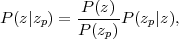(101)

so a photo-z that is is "unbiased" in the conventional sense of <z_p>|_z = z may still have δ z(z_p) ≠ 0. It is not required that photometric redshifts have δ z(z_p) = 0, but one does need to know the value of δ z(z_p) to relate observations to model parameters. From the simplified example discussed in Section 5.4.1, we can see that a systematic error of ~ 0.01 in δ z(z_p) / z_p will lead to a normalization error in the matter power spectrum of the order of 2%. Similarly, if 1% of galaxies in a source redshift bin z_s are actually outliers with redshift z ≪ z_s, they will dilute the expected lensing signal by 1%, and the power spectrum by 2%.

If the full distribution P(z|z_p) is known, then the shear cross-power spectra for any pair of redshift slices can be determined for a given cosmological model. However, the use of photo-zs to suppress intrinsic alignments (Section 5.6.1) does not work if the intrinsic alignments of the outliers are significant, or even if the scatter is large enough that galaxies can evolve significantly within a redshift bin, so there is a strong motivation to reduce them to the minimum level possible. Thus lensing programs must face two challenging problems: (i) obtaining a low outlier rate, and (ii) determining P(z|z_p) to sub-percent precision.

To understand how to reduce the outlier rate, we must investigate how photo-zs work: they take several broad-band fluxes from a galaxy and try to identify spectral features (see Fig. 18). At low redshifts, the strongest feature in the optical part of a galaxy spectrum is the break around 3800-4000E, arising from metal line absorption in early-type galaxies and the Balmer continuum (plus high-order lines) in late-type galaxies. As the redshift of the galaxy increases, this feature moves to the red, and above redshifts of z ~ 1.3 it is no longer useful for optical photo-zs (depending on the SNR in z and y bands). At z ≥ 2, the Lyα break redshifts into the optical bands and can be used - but it is possible to confuse it with the Balmer/4000E break. This is the principal example of a photo-z degeneracy.

Figure 18. The SEDs of three stellar populations are shown: a single burst at age 25 Myr (top); a continuous star-forming population of 6 Gyr age (middle); and a single burst at 11 Gyr (bottom). All have solar metallicity. Blueward of Lyα they have been adjusted for an IGM transmission factor of 0.8 (appropriate for z = 2.25; see McDonald et al. 2006), but other corrections (dust, nebular emission) are not included. The models are obtained from Bruzual and Charlot (2003). Note the break at ~ 0.37-0.40 μm present in all models, albeit with varying shape, strength, and precise location.

An alternative idea (Newman 2008) is to use the 2-D angular cross-correlation of the photo-z galaxies with a large area spectroscopic redshift survey, which can target brighter galaxies and/or the subset of faint galaxies that have strong emission lines. For a bin of galaxies with photo-z centered on z_p, the amplitude of cross-correlation is proportional to b_spec(z)b_phot(z, z_p)P(z|z_p), where b_spec and b_phot are the clustering bias factors of the spectroscopic and photo-z galaxies, respectively, at redshift z. The auto-correlations of the spectroscopic and photo-z samples provide additional constraints on the bias factors, and one also has the normalization condition ∫P(z|z_p) dz = 1 for each z_p bin. The key uncertainty in this approach is constraining the full redshift-dependent b_phot(z, z_p); if the bias varies with photo-z error (e.g., because high-bias red galaxies and low-bias blue galaxies have different photo-z error distributions) then this dependence must be modeled to extract P(z|z_p) (Matthews and Newman 2010). If one is using intermediate or small scale clustering, then one must also allow for scale-dependent bias and for cross-correlation coefficients lower than unity between different galaxy populations, which would lower the amplitude of cross-correlations relative to auto-correlations. Finally, the approach requires a spectroscopic sample that spans the full redshift range of the photometric sample; a quasar redshift survey may provide sufficient sampling density for probing the high-redshift tail of P(z|z_p). The cross-correlation technique has to date not been used for WL surveys, but it has been used to measure other redshift distributions — see, e.g., the application to radio galaxies by Ho et al. (2008). Adding galaxy-galaxy lensing measurements to the galaxy clustering measurements may improve the robustness and accuracy of the cross-correlation approach and allow some degree of "self-calibration" without relying on an external spectroscopic data set (Zhang et al. 2010).

Overall, the problem of measuring P(z|z_p) to the required accuracy remains one of the greatest challenges for future WL projects. Given the difficulty of assembling an ideal spectroscopic calibration sample, the treatment of photo-z distributions in Stage III and Stage IV WL analyses is likely to involve some combination of direct calibration, cross-correlation calibration, empirically motivated models of galaxy SEDs, and marginalization over remaining uncertainties in parameterized forms of P(z|z_p). Tomographic WL measurements themselves have some power to constrain these distributions (at the cost of some leverage on cosmological parameters), and weak lensing by clusters that have well determined individual redshifts may also be a valuable tool.

5.4.4. Lensing in the Radio

An interesting alternative to shape measurement in the optical is to work in the radio part of the spectrum, where late-type galaxies are observable via their synchrotron emission. In order to achieve the required resolution, one needs to use a large interferometer: a fringe spacing of 1" is achievable at 1 GHz with a baseline of 60 km. One also needs a large collecting area to obtain high-SNR images on a competitive number of galaxies; the SKA could in principle measure billions of galaxies (Blake et al. 2004). But let us suppose such an interferometer were built. What would it do for WL? In principle, it could solve many problems at once:

• Shape measurement: An interferometer directly measures the Fourier transform of the surface brightness of a galaxy, I(u), thereby avoiding the difficulty of interpolating PSF properties from stars. On long baselines, the u-plane is usually sparsely sampled, i.e., not all values of u are observed; the Fourier mode u = L_⊥ / λ, where L_⊥ is the interferometer baseline projected into the plane of the sky. At a given wavelength, as the Earth rotates, each baseline thus traces out an ellipse in the u-plane. However, if one combines a finite range of λ and many baselines, one could fill in the u-plane, and model-fitting shape measurement techniques can work even with significant coverage gaps. Model-fitting methods were used in the analysis of the FIRST survey at λ = 20 cm (Chang et al. 2004), which resulted in a 3σ detection of cosmic shear.
• Redshifts: Late-type galaxies contain atomic gas, and thus radiate in the H i 21 cm line. For nearby galaxies (z < 0.1) this line has a long history of being used as a redshift indicator. A Stage IV radio interferometer survey could collect hundreds of millions of spectroscopic redshifts in this line out to z~ 1-2, thereby obviating the need to rely on photo-zs and calibrate photo-z error distributions. Conversely, it is not clear that one could make use of the many radio galaxies not detected in H i, as even photometric redshifts for large radio galaxy samples are difficult to obtain at high completeness.
• Shape noise reduction: The radio part of the spectrum offers interesting opportunities to reduce shape noise. For example, if one spatially resolved the H i disk of a galaxy, one could produce a velocity map. A perfect inclined disk has the long axis aligned with the velocity gradient, and if sheared this alignment is destroyed, so a measurement of the velocity gradient provides independent information on the intrinsic shape of the galaxy (Morales 2006). Another idea is to use the polarization of the synchrotron emission, which tends to be perpendicular to the galactic disk and hence is an indicator of the position angle of the intrinsic minor axis (Brown and Battye 2011). While promising, these ideas are new, and their practical application to a WL survey may have to await at least a partial SKA.

5.4.5. Lensing of the CMB

It is also possible to do lensing analyses on the CMB. Here there are several advantages: the source redshift is known exactly from cosmological parameters, z_src = 1100; theory predicts exactly the statistical distribution of hot and cold spots on the CMB, so there is no intrinsic alignment effect; and the PSF (or "beam" shape) of microwave experiments tends to be far more stable than in the optical. The CMB is a diffuse field rather than a collection of objects (galaxies), so reconstructing the shear requires a different mathematical formalism than for galaxy lensing. The basis for this formalism is two-fold:

• In the presence of lensing by a Fourier mode of the potential ψ(l), the CMB anisotropy field is no longer statistically isotropic: different temperature Fourier modes become correlated, < T^∗(l₁) T(l₂)> ∝ ψ(l₂ - l₁). These products of temperature modes can be used as estimators of the lensing potential (Hu 2001).
• A more dramatic effect occurs for CMB polarization. The unlensed CMB polarization is pure E-mode, ⁴⁹ i.e., the polarization in each Fourier mode is parallel to the wavevector rather than at a 45° angle. Lensing shear changes the direction of the wavevector l but not the polarization, so it can generate B-mode shear.

Until recently, because of SNR issues, lensing of the CMB had been detected only in cross-correlation with foreground galaxies (Smith et al. 2007, Hirata et al. 2008, Bleem et al. 2012). The advent of the arcminute-scale CMB experiments ACT and SPT (primarily motivated by cluster cosmology using the SZ effect) has enabled robust detections of the power spectrum of the CMB lensing field (Das et al. 2011, van Engelen et al. 2012).

Because CMB lensing only provides a single source slice, it is unlikely to ever replace galaxy lensing. However, in combination with galaxy lensing, it can provide the most distant source slice for tomography (Hu 2002b) and cosmography (Acquaviva et al. 2008).

5.5. Measuring Shears

So far we have treated shear measurement as a black box: it takes in an image of the galaxy and some knowledge of the instrument, and it returns γ_+,W, an unbiased estimator for the true shear γ with some uncertainty per component σ_γ. This black box is very complicated on the inside, as one needs an accurate and robust shape measurement algorithm, and even providing the necessary inputs to such an algorithm, particularly an accurate determination of the PSF, has proven to be difficult. After a brief overview of these algorithms, we describe the idealized problem of measuring shear from an ensemble of galaxy images, then turn to a more detailed discussion of the challenges that arise in practice.

There are two general strategies for shape measurement methods in common use today. One class of methods is to measure moments of galaxies (in real or Fourier space), and relate, e.g., the mean quadrupole moment of galaxies to the shear. These methods started with ad hoc "PSF correction" prescriptions, but they have recently evolved toward methods that attempt to statistically close the hierarchy of moments of galaxies and PSFs in a model-independent way. The other class of methods is based on forward modeling: one adopts a model for a galaxy (e.g., an elliptical Sersic profile, or a linear combination of basis images), simulates the observational procedure, and minimizes χ². Both approaches have their advantages and disadvantages. Much of the early WL work used moments-based methods, but for years a generally applicable PSF correction scheme seemed out of reach. Some of the more recent incarnations of the Fourier domain moments-based methods work for arbitrary distributions of galaxy and PSF profiles; however these are less mature in their practical implementation, and they impose stringent requirements on input data quality (e.g., sampling). The forward modeling methods can handle a much wider range of observational defects (e.g., under some circumstances one may even be able to measure a galaxy containing missing pixels), but they depend on a model for the galaxy being observed; one must carefully assess the impact of an insufficiently general model. Both strategies require exquisite knowledge of the PSF.

Currently there are many algorithms in use in each category. The prototype moments-based method was that of Kaiser, Squires, and Broadhurst (KSB; Kaiser et al. 1995; improved by Luppino and Kaiser 1997, Hoekstra et al. 1998). Many improvements of these methods have been made — e.g., in computing better conversion factors from shear to quadrupole moments ⁵⁰ (Semboloni et al. 2006b). Elliptical-weighted moments and the concept of shear-covariance were introduced by Bernstein and Jarvis (2002) and have been used extensively in SDSS (Hirata and Seljak 2003b). Further progress was made by moving to moments in Fourier space, where the PSF "correction" becomes trivial (one divides by the Fourier transform of the PSF, at least in the regions where it is nonzero). This has culminated in the development of a shape measurement method that is exact in the high-SNR limit (Bernstein 2010). We discuss this method and its development in Section 5.5.2. An early example of the model-fitting approach was im2shape (Bridle et al. 2002). More recently, Bayesian model fits have been introduced that are stable at lower SNR (Miller et al. 2007, Kitching et al. 2008); these are currently being applied to the CFHTLS. The "shapelet" basis (Refregier 2003, Refregier and Bacon 2003), derived from energy eigenstates of a 2D quantum harmonic oscillator, is useful in both types of methods. The coefficients in a shapelet decomposition are moments, but one may also fit a model galaxy parameterized by its shapelet coefficients.

The various shape measurement algorithms have been tested and compared in blind simulations, such as the Shear Testing Program (STEP1/STEP2; Heymans et al. 2006, Massey et al. 2007a), GREAT08 (Bridle et al. 2010), and GREAT10 (Kitching et al. 2010). In most of these cases, the objective is to minimize both the shear calibration error m (i.e. the error in the response to a given input shear) and the spurious shear c (i.e., the shear measured by the algorithm on an unlensed sample of galaxies). The STEP2 simulations used typical ground-based PSFs and complex galaxy morphologies and found that many of the measurement methods had shear calibration errors |m| of one-to-several percent, and spurious shear |c| ranging from several × 10^-4 to several × 10^-3. This level of performance should thus be considered typical of the more mature, heavily used shear measurement algorithms, although recent methods have done better. On the other hand, the algorithmic errors are only a portion of the error budget in a WL experiment — most importantly, the early simulation tests did not require participants to recover the spatial variability of the PSF. Such a test is currently ongoing as part of the GREAT10 challenge (Kitching et al. 2010). Early results from GREAT10 are now available, but their significance is still being digested.

In the remaining portions of this section we will discuss the mathematical problem of shape measurement (Section 5.5.1) and the basis for some of the commonly used methods (Section 5.5.2) and their statistical errors (Section 5.5.3). We cannot of course do justice to every method that has been suggested or used. We have chosen to highlight the recent progress in Fourier-space methods, since in principle they provide an exact solution in the limit of high SNR and are thus ripe for further development and utilization (Bernstein 2010). There are some biases that can result even for perfect shape measurement (or galaxies measured with a δ-function PSF), including the noise-related biases and selection biases, which are probably present at some level for all known algorithms; these are discussed in Section 5.5.4. Finally Section 5.5.5 describes the determination of the PSF, which is taken as an input for any shape measurement algorithm.

5.5.1. The Idealized Problem

The idealized shape measurement problem is as follows: we have a galaxy in the source plane whose surface brightness is f₀(x), where x is a 2-dimensional vector in the plane of the sky. It is first sheared, i.e., the galaxy in the image plane is f(x) = f₀(Sx), where S is the shearing matrix,

(102)

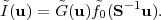
(We assume |γ| ≪ 1 here and work to linear order in γ for simplicity, although higher-order corrections will be important for Stage IV surveys.) We do not observe the actual image on the sky, however — we observe it through an instrument with PSF ⁵¹ G(x). The resulting image is

(103)

This equation may also be written in Fourier space: if we define

(104)

then equation (103) simplifies to

(105)

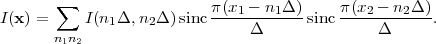
In practice, the image I is only obtained at discrete values of x, i.e., at the pixel centers spaced by separation Δ. If the image is oversampled, i.e., if the Fourier transform ⁵² of the PSF is zero (or negligible) at wavenumbers above some |u|_max with |u|_max < 1 / (2Δ), then it can be sinc-interpolated to recover the full continuous function,

(106)

The pixelization thus represents no special difficulty, except that the sinc function has noncompact support and must be smoothly truncated. A second implication of oversampling is that integrals of the form ∫P(x) I₁(x) I₂(x) d²x, where P is a polynomial in the coordinates and I₁ and I₂ are oversampled functions, can be replaced without error by (infinite) sums over pixels: ∫ → Δ²Σ. Again, in practice such sums must be truncated.

We will also define a critical wavenumber u_crit, which is the smallest wave number for which there is a Fourier mode with G(u) = 0 with |u| = u_crit. Then we have G(u) ≠ 0 for any |u| < u_crit. This critical wavenumber determines the region within the Fourier plane over which deconvolution is possible, and over which measurement of f(u) is possible.

A shape measurement algorithm is a functional γ_i[I;G], i ∈{+,W}, that returns a shear estimate. When averaged over a population of galaxies with the same shear, such an algorithm will yield an expectation value

(107)

Here c_a is called the additive shear error and m_ab is the multiplicative shear error or shear calibration error. An ideal algorithm will have c_a = m_ab = 0.

Many WL surveys take multiple exposures of each field; if they are oversampled, one may use equation (106) to reconstruct a continuous function I(x) for each exposure. If the PSFs in each exposure differ (which they usually do), then to construct a stacked image, one can either apply a convolution kernel to each input image to make the PSFs the same or do a noise-weighted least squares fit to each Fourier mode f(u). If the individual exposures are undersampled (as is likely for space-based data) and appropriately dithered, methods are available in both Fourier space (Lauer 1999) and real space (Fruchter 2011, Rowe et al. 2011) to reconstruct a fully-sampled and hence continuous image I(x). ⁵³ In either case, the problem is still one of measuring the shear from an ensemble of images of different galaxies. The one exception is that model-fitting shape measurement techniques can operate either on the combined images or via a direct fit to the raw input images. Even in this case, however, with many exposures (as planned for LSST) object detection will have to be carried out on the combined image in order to reach the full survey depth.

One would intuitively expect that shape measurement becomes more difficult when the PSF is larger than the intrinsic size of the galaxy being measured. This is indeed the case. While the idealized problem of measuring shapes in the presence of a PSF is well-defined for any nonzero galaxy size, in practice both statistical and systematic errors blow up when the PSF becomes significantly larger than the galaxy. The extent to which the systematic errors in the high-SNR, r_gal < r_psf regime can be addressed will likely determine the constraining power of large-itendue ground-based WL programs such as that planned for LSST.

5.5.2. Shape Measurement Algorithms*

The most obvious — but flawed — way to construct a shape measurement algorithm is to simply use the quadrupole moment tensor of a galaxy: one could compute

(108)

where is the centroid and the [I] implies that we compute the quadrupole moment on an observed image. It is easily seen from the properties of convolutions that Q_ij[f] = Q_ij[I] - Q_ij[G], i.e., one may obtain the pre-PSF quadrupole moment of a galaxy by subtracting the observed quadrupole moment from that of a PSF. Then one could construct the ellipticities of the galaxy, which are simply the trace-free components of the quadrupole moment normalized by the trace:

(109)

Since the quadrupole moment of f is simply related to that of f₀ via

(110)

we may derive the transformation law for ellipticities under infinitesimal shear:

(111)

It is then easily seen that the mean ellipticity of a population of galaxies that has an initially isotropic distribution of ellipticities - i.e., P(e₊, e_W) depends only on the magnitude (e₊² + e_x²)^1/2 and not on the direction arctan(e_x / e₊) — is

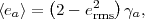(112)

where e_rms² is the mean square ellipticity per component (+ or ×). Since we work to first order in γ, we may use the mean square ellipticity of the observed sources in equation (112). So the galaxy ellipticity divided by 2 - e_rms² is a shear estimator satisfying our desired conditions: by comparison to equation (107) there is no additive or multiplicative bias.

The problem with this procedure is that the unweighted quadrupole moment, equation (108), involves an integral over the entire sky, with a weight that increases ∝ x² as one moves away from the centroid of the galaxy. Therefore its measurement noise is infinite. It also fails to converge if the wings of the PSF decline as G(x) ∝ |x|^-α for α ≤ 4, i.e., it fails to converge for all PSFs realized in modern optical telescopes. Therefore equation (108) needs modification.

A conceptually simple approach is to do a model fit to each galaxy. If one fits a model of an exponential or de Vaucouleurs profile galaxy with homologous elliptical isophotes, then one can obtain the quadrupole moment Q_ij[f] analytically from the model and hence the ellipticity of the galaxy. Modern model-fitting techniques can even fit more general radial profiles, or simultaneously fit bulge + disk models. Model fitting is also robust against many types of nastiness that occur in real data, such as dead pixels, cosmic rays, or nonlinear detector effects. However, model fitting assumes that the galaxy actually obeys the model — and especially at z > 1, the appearance of galaxies is not simple and they are not describable by simple analytical functions. At present, our best approach to understand what happens when simple model fits are confronted with complex galaxies is with simulations. One can even imagine "re-calibrating" these methods using the simulations, e.g. by subtracting the simulated c_i from each shear and multiplying by the matrix inverse of δ_ij + m_ij (see eq. 107); but of course one is then relying on the galaxy population in the simulation to closely trace reality.

One could also attempt to do a regularized deconvolution of the galaxy. The most popular such technique is a basis function technique: one writes the galaxy image as f(x) = Σ_n b_n ψ_n(x), where {ψ_n} are a finite basis set and b_n are the fit coefficients; this then becomes a model-fitting problem. A common choice is the "shapelet" basis, where the {ψ_n} are the energy eigenmodes of the 2-D quantum harmonic oscillator (polynomials times Gaussians); this requires (N + 1)(N + 2) / 2 eigenfunctions to represent the 0...N energy levels (Refregier 2003, Refregier and Bacon 2003). This basis is complete in the limit of large N, and the Gaussian endows the basis coefficients with simple transformation properties under translation and shear. Real galaxies often require very large N to be well-represented, however, especially for cuspy profiles.

A final class of ideas has been to note that any ellipticity formula that is shear-covariant in the sense of transforming via equation (111) enables us to use equation (112). For example, suppose that we had the galaxy image f before PSF convolution, and did an unweighted least-squares fit, in the sense of minimizing

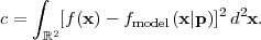(113)

Here f_model is an elliptical Gaussian fit to the image with free amplitude A, centroid _i, and second moment matrix Q_ij^elfit (6 parameters). Then Q_ij^elfit and the ellipticities constructed from it would be shear-covariant — even if the galaxy's true radial profile does not resemble a Gaussian! ⁵⁴ Early work on implementing this idea in the presence of a PSF attempted to determine the second moment matrix of the image on the sky Q_ij^elfit[f] from the observed image and the PSF. For example, Gaussian galaxies and PSFs satisfy Q_ij^elfit[f] = Q_ij^elfit[I] - Q_ij^elfit[G], and so "non-Gaussianity corrections" were introduced (Bernstein and Jarvis 2002, Hirata and Seljak 2003b) that yielded shear calibration errors of a few percent. But these methods were heuristic, and moreover they suffer from a fundamental limitation: Q_ij^elfit[f] depends on very high-wavenumber Fourier modes u of the image, which are not preserved by the PSF, i.e. G(u) = 0. It is therefore mathematically impossible to determine Q_ij[f] from the data in a model-independent manner.

To understand this point more fully, and illustrate a solution, let us imagine that we are doing an unweighted least-squares fit of a parameterized image f_model(p), using equation (113). For convenience, we will write the parameters as p = { A, σ_gal, ₁, ₂, e₊, e_W}, where σ_gal = (detq)^1/4 is a characteristic scale length of the galaxy, so that they have simple transformation properties under rotations. Written in Fourier space, it becomes

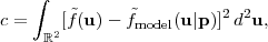(114)

and its minimum is given by the simultaneous solution of the 6 equations

(115)

where p_α is any of the 6 parameters. The problem occurs because ∂ f_model(u|p) / ∂ p_α has support at |u|>u_crit, where we cannot determine f(u).

A solution to this problem has been proposed by Bernstein (2010) ⁵⁵, which is in principle exact in the low-noise limit and has been applied to simulations (but not yet to actual data). The key is to work in the Fourier domain, where the effect of the PSF is simple and the effect of the shear is as simple as in real space. We present the solution here in its most general form, and refer the reader to Bernstein (2010) for implementation details. The solution is to replace equation (115) with

(116)

where W₁...W₆ are weight functions. These should be envisioned to be qualitatively similar to the derivatives in equation (115); but the only rules that we will impose are that: (i) the Fourier transforms W_α(u|p) have compact support, confined to |u| < u_crit; and (ii) they are rotation and translation-covariant, e.g., changing the centroid parameter by δ simply translates the function W_α(x) → W_α(x - δ), and there is a similar transformation when rotating the ellipticity components. ⁵⁶ We do not require the W_α to be shear-covariant: indeed, since a large shear can map any mode to another mode with |u| > u_crit, such a requirement would be inconsistent with rule (i). Now we may write equation (116) as

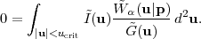(117)

The combination W_α / G is well-defined, and I(u) is the Fourier transform of the observed image, so the parameters p can be measured from the data.

By rule (ii), we have rotation covariance, so the mean of the ellipticities ⟨e⟩ over an isotropic population of galaxies is zero — even if the PSF is anisotropic. Thus there is no additive bias (except for selection and noise effects — see warnings below). However, dropping shear covariance has come at a price: the ellipticities (e₊, e_W) no longer transform according to equation (111), and the responsivity coefficient <e> = γ must be determined. Fortunately, we can evaluate the effect of an infinitesimal shear on equation (116): if S = 1 + δS, then to first order in δS,

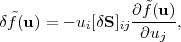(118)

and so

(119)

The integral in braces {} is simply a 6 × 6 matrix, which we denote E_αβ. Using integration by parts, the tracelessness of δS in the first integral, and the substitution f → I / G, we then find

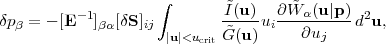(120)

which is well-defined. This equation tells us how the parameters for each galaxy vary under an infinitesimal shear; their ensemble average gives . Note that once shear covariance has been dropped, it is only possible to know the responsivity factor if one has a sample of real galaxies to observe, since one needs the sample of real galaxies to compute the matrix E_αβ.

A related approach to solving the shear calibration problem was suggested by Mandelbaum et al. (2012). They noted that given a high-resolution image of a galaxy (e.g., a space-based image) with PSF G₁, it is often possible to construct a lower resolution but sheared image of the same galaxy with PSF G₂ in a model-independent way. One can thus directly test any shear estimator on the sheared images, and extract the shear calibration factor. Conceptually, the criterion for this to work is that all of the Fourier modes of the image observable using PSF G₂ must be within the band limit of G₁ with enough "padding" to make sure that the shear (which also shears the Fourier plane!) does not bring unobserved high-wavenumber modes not seen with G₁ into the region seen by G₂. Mathematically, the criterion for this to be possible are that there exist two critical wavenumbers u_c and u_d such that (i) all the power in the low-resolution PSF is below u_c, i.e. G₂(u) = 0 for |u| ≥ u_c; (ii) the high-resolution transfer function G₁(u) is far from zero, i.e. 1/ G₁(u) is well-behaved, at all |u| <u_d; and (iii) u_c > (1 - γ)u_d. Then one can use the Fourier-domain multiplication:

(121)

where T(u) = 1 / G₁(u) for wave vectors |u| < u_d. As implemented, this method requires a higher-resolution image of a fair subsample of galaxies, which is not always available. It may however be quite useful in the Stage III ground-based programs, where one might use HST data for the "high resolution" image; see Mandelbaum et al. (2012) for a preliminary application of HST data to shear calibration in SDSS.

5.5.3. Shape Measurement Errors*

The statistical uncertainty in ellipticity estimation depends on the method used and the radial profile of the galaxy, as well as the sizes of the galaxy and PSF and the SNR. Rules of thumb can be obtained by considering nearly circular Gaussians. Propagating instrument noise through the elliptical Gaussian fitting method, Bernstein and Jarvis (2002) find, in the absence of a PSF,

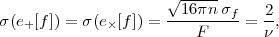(122)

where n is the flux noise variance per unit area, F is the galaxy flux, σ_f is the 1σ width of the galaxy (note: the effective radius of a Gaussian is 1.177 σ_f), and ν is the detection SNR in an optimal filter. In the presence of a circular Gaussian PSF, the ellipticity is diluted by

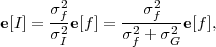(123)

where σ_g is the PSF width and σ_i is the width of the PSF-convolved galaxy image. Furthermore, the detection SNR is reduced because the galaxy is smeared out into an aperture with more noise, so it follows that equation (122) should be modified by replacing σ_f → σ_i; and, if we want the uncertainty in the pre-PSF galaxy ellipticity, we must divide out the σ_f² / σ_i² factor from equation (123). This gives

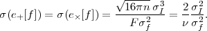(124)

This provides a large advantage for making the PSF smaller than the galaxy: since the noise variance n scales with observing time as t^-1, the time required to measure the shape of a galaxy scales as

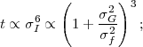(125)

in the limit of a poorly resolved galaxy (σ_f ≪ σ_g) a factor of 2 improvement in the PSF provides a factor of 64 gain in speed. However, as the PSF becomes smaller than the galaxy this advantage saturates.

Equation (123) also illustrates another property of shape measurement: systematic errors as well as statistical errors are inflated by having large PSFs. For example, if there is a systematic error in the ellipticity of the observed image I, it propagates to the estimated pre-PSF ellipticity e[f] with a multiplying factor of (σ_f² + σ_g²) / σ_f². Therefore there is a systematics advantage to having σ_g ≪ σ_f.

The shear uncertainty is a factor of ~ 2 smaller than the ellipticity uncertainty owing to the responsivity factor 2 - e_rms² (eq. 112). It does however have a minimum value: the ellipticity of an individual galaxy has an RMS variation of e_rms ~ 0.4 per component, so there is a limiting "shape noise" contribution to the shear measurement uncertainty of σ_γ ≈ 0.2. There are some ideas for how to circumvent this limit using the color- or scale-dependence of ellipticity (Lombardi and Bertin 1998, Jarvis and Jain 2008) or taking advantage of the non-Gaussianity of the ellipticity distribution (Kaiser 2000, Bernstein and Jarvis 2002), but there are no clear routes to large improvement for optical galaxies. For galaxies imaged in the HI 21cm line, one might be able to use kinematic signatures to distinguish random orientation from lensing shear (e.g. Morales 2006).

5.5.4. Noise Rectification and Selection Biases*

Two pernicious biases can arise even for the "exact" shape measurement algorithms described above: the noise rectification and selection biases.

Noise rectification bias arises whenever a nonlinear transformation, such as ellipticity measurement, is applied to noisy data. If we Taylor-expand the mean of the ellipticity measured on the true image I_obs around the noiseless image I, we find

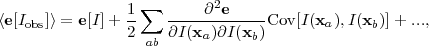(126)

where the sum is over pairs of pixels in the image, and x_a and x_b are positions of those pixels. The bias is proportional to the noise variance, i.e., to (S / N)^-2 at leading order.

One might at first think that the pixel covariance is described by uncorrelated white noise, which is statistically shear-invariant and thus leads to no bias, but in the presence of a PSF correction [i.e., dividing by G(u)] this is no longer the case. The noise rectification bias was first recognized in the context of WL by Kaiser (2000), who showed that because the centroiding of a galaxy is more accurate on the "short" than the "long" axis of the PSF there is a preference for the measured second moment of the galaxy to be elongated along the PSF, even if the PSF correction method is perfect in the deterministic case. This was generalized by Bernstein and Jarvis (2002) to incorporate other noise-related biases and by Hirata and Seljak (2004) to include the effect on shear calibration errors. Equation (126) provides a unified framework for computing all of these biases to order (S / N)^-2. At low S/N higher-order terms in the expansion may become important, and the expansion itself may break down, e.g., as fitting algorithms jump to alternate χ² minima. It is our judgment that it is best to stay away from this "nonperturbative noise" regime. For a recent investigation of noise rectification bias in the context of current shape-measurement algorithms, see Melchior and Viola (2012).

Selection biases are well-known in astronomy. In our case, they will affect the shear if there is a bias in favor of detecting galaxies in some orientations rather than others, producing an additive shear error, or if selection depends on the magnitude of the ellipticity, which leads to a multiplicative shear error because galaxies are preferentially selected when their intrinsic ellipticity is aligned with the shear (Hirata and Seljak 2003b). A similar bias results if galaxies are weighted by various properties (e.g., ellipticity uncertainty) that are not shear-invariant. The formalism of Section 5.5.2 can in principle handle this problem if instead of computing <e> we compute <we> where the weight w = 0 for galaxies that are rejected. However, the assessment of selection biases in practice has been addressed through simulations such as the STEP program.

A problem related to selection biases is blending: the superposition of images of two galaxies. If the galaxies are at the same redshift, they are affected by the same shear, and an ideal shape measurement algorithm that measures the blend should recover the "correct" answer — indeed, existing WL surveys must contain many sources that are actually blended with their own satellite galaxies. But if the deblending algorithm is not shear-invariant there can be a bias in the shear. Another issue, particularly for ground-based Stage IV experiments that will aim for high source densities at modest resolution and very small statistical errors, is accidental blending of galaxies at different redshifts (and hence different shears).

The general strategy for dealing with these categories of biases is: (1) make choices (e.g., S/N cuts) that keep them small to the extent possible; (2) compute corrections using simulations and/or analytic estimates, and apply them to the measurements; (3) test the accuracy of these corrections in the data by looking for the expected scalings with S/N, source size, and so forth; and (4) marginalize over remaining uncertainties in the corrections.

5.5.5. Determining the PSF and Instrument Properties

Shape measurement algorithms are only as useful as their inputs: in this case a map of the PSF G(x) at each point in the field. Determining the PSF to sub-percent accuracy is one of the major challenges in WL. Errors in the PSF model introduce correlated structure into the ellipticity field of the galaxies, since residual anisotropy in the PSF determination is interpreted as shear by a shape measurement algorithm.

Fortunately, Nature has provided us with stars, which under typical observing conditions can be treated as point sources. Unfortunately, there is only a finite density of stars in high Galactic latitude fields, typically of order 1 per arcmin², so one must interpolate the PSF to the position of a galaxy. This is a demanding challenge; any error in the interpolated PSF is likely to have spatial structure. It is also not an easy problem, as the PSF is an entire function G(x; θ) at every 2-d position θ on the sky, and in contrast to shape measurement, interpolation from stars is underconstrained. ⁵⁷ To date, most of the methods applied to real data are heuristic. For example, the SDSS analyses fit a low-order polynomial,

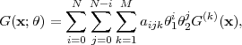(127)

where the {G^(k)} are the top M = 3 principal components of the stellar images, N = 2 is the interpolation order, and a_ijk are coefficients. Small scale structure in the PSF variation may not be well represented by this approach unless N is large, but if the required number of polynomial coefficients (N + 1)(N + 2) / 2 exceeds the number of stars in each frame then the method falls apart. If the small-scale structure is repeatable, for example if it is associated with low-order aberrations in the telescope or the topography of the focal plane, then one may make progress by applying PCA to the angular dependence in instrument-fixed coordinates (Jarvis and Jain 2004), choosing the top K modes out of the space of (N + 1)(N + 2) / 2 polynomials. Recent work has focused on improved interpolation schemes that outperform polynomials (e.g., Bergi et al. 2012).

For space-based data, one can either build a physical model of the PSF (Rhodes et al. 2006) or use PCA (Jee et al. 2007). However, for ground-based data where the PSF has a large contribution from atmospheric turbulence, the more empirical interpolation schemes have been the methods of choice.

Once one has the PSF, one needs a method of quality assessment. We need to be able to determine, or at least bound, the power spectrum of the residual PSF systematics that leak into cosmic shear results. (For GGL, this job is easier because residual PSF anisotropy adds noise but does not correlate with the positions of the galaxies.) One way is to do null tests: one can compute the correlation function of ellipticities of the stars and (supposedly) PSF-corrected galaxies, or search for B-mode shear. The latter is not foolproof, as a PSF systematic of E-mode type can arise from some aberrations. A very attractive (but underutilized) test is to mask some of the stars in the PSF fitting and compare the interpolated PSFs at their locations to the observed stellar images. There are also methods for using combinations of these correlation functions to test for "overfitting" - the phenomenon in which a too-general PSF model begins to fit noise or small-scale structure in the stellar images, with the effect that the interpolated PSF is actually worse (Rowe 2010).

Even when this is done, there remain two other errors that have received increasing attention recently, which may cause the PSF of a galaxy to differ from that of a star:

• Color dependence: Real PSFs depend on the wavelength of light: a diffraction-limited telescope has a PSF size that scales ∝ λ, seeing through a Kolmogorov atmosphere gives a size ∝ λ^-1/5, aberrations introduce λ-dependence into not just the size of the PSF but its morphology and radial profile, real detectors have response functions that depend on wavelength, and in ground-based data atmospheric dispersion acts like a prism and causes a centroid shift with wavelength. Since galaxies have different SEDs than the stars used to fit the PSF (the galaxies are usually redder), the PSF measured from the stars is not always appropriate to the galaxies (Cypriano et al. 2010). Moreover, each galaxy contains a range of SEDs due to differing stellar ages and metallicities and dust columns; and for each of these SEDs there is a different PSF, with the resulting images superposed on the focal plane (Voigt et al. 2012). This represents a major challenge: while the centroid wavelength of galaxies in a typical filter (λ / Δλ ~ 5) varies by several percent, Stage IV surveys will require sub-percent shear calibration accuracy, and as yet no WL survey has published a color correction to its PSF at all. While this area requires much more work, in a problem of this complexity prevention is the first step to a cure. For example, one can employ an atmospheric dispersion compensator on the ground, and one can use narrower filters. For smooth spectra or spectra averaged over moderate redshift ranges, the variation of wavelength centroid scales as ∝ Δλ². The advantage for narrower filters must of course be weighed against the slower survey speed with smaller Δλ. If many observations of a given field are taken under varying conditions, as planned for LSST, one has the intriguing possibility of using the different seeing, focus, or hour angle dependences of these errors to solve them out and distinguish them from shear. A final strategy is to use "calibration samples" of galaxies observed in multiple filters to correct the effect for a lensing survey with a single, wide band (Semboloni et al. 2012).
• Detector effects: A CCD image can be altered during readout due to finite charge-transfer inefficiency. This results from photoelectrons that temporarily bind to defects ("traps") in the material, causing each sky object to leave a trail along the readout direction. If not corrected, this can appear as a PSF anisotropy, and it is greater for faint objects than for bright objects because some of the traps saturate, so stellar images tend to underestimate the effect. Charge transfer inefficiency is primarily a concern for space-based data, since the principal cause of traps is radiation damage. Remedies applied to HST data have included empirical corrections to the galaxy ellipticities as a function of row and magnitude, or pixel-level corrections that begin by "undoing" the charge transfer inefficiency before subsequent processing (Massey et al. 2010, Rhodes et al. 2010).
• Near-infrared detectors (as planned for WFIRST) suffer from different potential detector-induced systematic errors than CCDs. In particular, since the image is read "in place" on the detector rather than transferred out as on a CCD, there is no charge transfer inefficiency. Instead the major concerns have been interpixel capacitance (the sensitivity of the voltage on each pixel to the charge collected in neighboring pixels); persistence (a charge trapping and release phenomenon in which each exposure contains a small amount of residual signal from previous exposures); and reciprocity failure (a detector exposed to twice the signal for half the time does not produce the same response, which becomes an issue for comparing the images of stars and galaxies of very different magnitudes).

5.6. Astrophysical systematics

The principal advantage of weak lensing is that — despite its technical difficulty — it is directly sensitive to mass. It is thus less affected by astrophysical uncertainties than other probes of cosmic structure such as the galaxy power spectrum or X-ray cluster counts. However, it is not entirely free of astrophysical contamination. The two major sources of uncertainties in this case are intrinsic galaxy alignments, which can mimic the coherent distortion of galaxies by gravitational lensing, and the prediction of the matter power spectrum.

5.6.1. Intrinsic Alignments*

We have thus far assumed that the intrinsic ellipticities of galaxies are independent, adding noise but not spurious signal to cosmic shear measurements. However, the orientations of galaxies are determined by physical processes — mergers, torquing by tidal fields from the host halo and large scale structure, etc. — that could produce correlated intrinsic alignments. We first describe here the general formalism for the impact of intrinsic alignments, then consider what observations and theory have taught us about them. We conclude by discussing prospects for intrinsic alignment removal.

The field of intrinsic galaxy ellipticities is a tensor function e(r, ) of position r and viewing direction . In this sense it is very similar to CMB polarization. In principle it also depends on the type of galaxy under consideration and on the observational details — for example, the B and I-band images of a galaxy could have different ellipticities. We may also discuss either the unweighted intrinsic ellipticity field e_unwt or the field weighted by the galaxies,

(128)

where g = (n_gal - ) / ) is the galaxy overdensity. In what follows, we use e to denote the galaxy-weighted field e_wt, since this is most closely related to what one observes in a survey.

Like any other field, e can be Fourier transformed to give e(k, ), with a power spectrum

(129)

where a, b are spin-2 tensor indices. Here we break from the train of reasoning in CMB polarization studies: instead of doing a multipole decomposition of e, we note that in the Limber approximation (which we use exclusively here) there is only one relevant viewing direction - the direction to the observer — so = '. Moreover, the Fourier wave vectors that we care about are perpendicular to the line of sight, so k ⋅ = 0. We will thus write this particular configuration as simply P_e;ab(k). An E / B mode decomposition is also possible if we rotate the coordinate basis so that the E-component of ellipticity is aligned along the direction of k and the B-component is at a 45° angle; we then have two ellipticity power spectra, P_e^EE(k) and P_e^BB(k) (the EB-term vanishes by parity). One can also write correlations of the ellipticity with scalar fields such as the galaxy or matter density. In this case, only the E-mode can be correlated, and we write P_eδ, P_eg, etc.

The measured shear on the sky is a superposition of the WL shear and the intrinsic ellipticity (converted to shear using the algorithm-specific responsivity factor ):

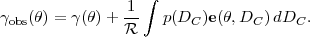(130)

Limber's equation can then be used to obtain the observed shear power spectrum between the α and β redshift slices. The E-mode contains three terms:

(131)

where the GG term is the gravitational lensing shear contribution, II is the intrinsic ellipticity contribution, and GI is the cross-correlation. The GG term is the desired signal and is given by equation (81). The other terms are

(132)

and

(133)

There is also an II contribution to the B-mode power spectrum similar to equation (132). Since there is no B-mode gravitational shear, there is no GG or GI contribution to the B-mode power spectrum.

Several generic features can be noted from these equations:

• The II contribution to the cross-spectrum is only nonzero if the two redshift distributions overlap, since it arises from intrinsically aligned galaxies at the same redshift. Therefore, if low-scatter photo-zs are available, it can be eliminated. This is one motivation for doing tomography instead of simply measuring the shear power spectrum on a magnitude-limited sample of galaxies.
• The GI contribution is more troublesome. It arises from the lensing of the more distant slice by the same matter field that controls the intrinsic ellipticity of the nearby slice. Inspection of the properties of the window function W_eff shows that equation (133) is nonzero for all redshift distributions, unless either P_eδ(k) = 0 or the redshift distributions are δ-functions at the same redshift, which would dramatically enhance II. Thus we are led to conclude that every tomographic power spectrum can suffer intrinsic alignment contributions.
• B-mode "shear" can be generated by intrinsic alignments, and if nonzero C_BB^αβ(l) is observed this is one possible explanation (PSF model errors are another). However, it is possible for the intrinsic alignment contribution to the E-mode to be much larger because (i) there is no theoretical reason from galaxy formation to expect P_e^EE(k) ~ P_e^BB(k) — indeed, we will see below that P_e^EE(k) ≫ P_e^BB(k) may be natural — and (ii) C_EE^αβ(l) can also contain a GI term, which for broad redshift distributions usually dominates over II. Therefore a nondetection of B-mode shear does not rule out significant intrinsic alignment contamination.

Before we discuss removal of intrinsic alignments, it is helpful to consider the physics underlying their power spectra. One can distinguish two cases: early-type galaxies, which are triaxial and whose intrinsic ellipticity is presumably related to the direction of the most recent merger or the direction of anisotropic collapse (depending on one's idea of how these galaxies are formed), and late-type galaxies, whose ellipticity is determined by the disk angular momentum (perhaps acquired via tidal torquing during collapse, reshuffled by disk-halo interactions, and perturbed by minor mergers). The detailed physics of these processes remains elusive, but some predictions can still be made by traditional galaxy biasing arguments. For example, if one considers the formation of early-type galaxies in a particular region of the universe, one could argue that at linear order in the large-scale density field a galaxy's formation sequence can be sensitive only to the density and tidal field coming from the linear modes, and to small-scale structure. Since only the tidal field has the correct symmetry properties to be related to an ellipticity, it follows that the ellipticity should be proportional to the tidal field,

(134)

where C₁ controls the strength of alignment and ∂₁ and ∂₂ denote derivatives along two orthogonal axes on the sky. This implies that the ellipticity traces the density field, and in particular

(135)

Equations (134, 135) are known as the linear alignment model (Catelan et al. 2001). Note that they predict only E-mode intrinsic alignments, because the alignments are linearly sourced by a scalar field. ⁵⁸

Observations of LRGs in the SDSS have shown that the galaxy-ellipticity correlation ⁵⁹ w_ge(r_p) has the same power-law slope as the galaxy correlation function w_g(r_p) ∝ r^-0.7 (Mandelbaum et al. 2006, Hirata et al. 2007), with an amplitude that increases rapidly with LRG luminosity. This is a quantitative success of the linear model. However, on small scales it is not clear how accurate equation (135) should be.

For late-type galaxies, it is less clear what to expect. The oldest and most widely discussed model is that disk galaxies acquired their angular momentum from tidal fields acting on nonspherical protogalaxies, an effect that would make the resulting intrinsic ellipticity quadratic in the tidal field: this is known as the quadratic alignment model (Pen et al. 2000). This model produces both E and B-mode II signals, but to leading order it predicts P_eδ(k) = 0 and hence gives no GI signal (Hirata and Seljak 2004). However, one should be cautious about this argument for several reasons, most importantly because there has not yet been any quantitative observational confirmation of the scale and configuration dependence predicted by the quadratic model, and additionally because perturbation theory arguments show that the nonlinear evolution of the tidal field can generate a linear type alignment (Hui and Zhang 2008). What is clear from observations is that the alignments of late-type galaxies on large scales, at least as measured by w_ge(r_p), are consistent with zero and are certainly much less than for LRGs (Hirata et al. 2007, Mandelbaum et al. 2011).

Detailed assessments of the intrinsic alignment contamination have been made on the basis of SDSS, 2SLAQ, and WiggleZ observations of w_ge(r_p) (Hirata et al. 2007, Mandelbaum et al. 2011, Joachimi et al. 2011). These studies show that for surveys of modest depth (z_med ~ 0.7) the GI contamination may be up to several percent of the expected cosmic shear signal for late-type galaxies if it is near current upper limits, and it could be tens of percent for LRGs. As one probes to higher source redshifts the level of contamination becomes increasingly uncertain, because there are not yet galaxy surveys at z ≥ 1 that are capable of probing intrinsic alignments at interesting levels. The II contamination for broad redshift distributions is found to be much less than GI for linear alignment models.

Finally, we consider the methods used to remove intrinsic alignments. One starts with prevention: in the recent COSMOS analysis, Schrabback et al. (2010) suppressed II by throwing out the auto-power spectra of each of their redshift slices with itself, keeping only the cross-spectra. They also suppressed GI by not including LRGs in the foreground redshift slice, since LRGs contribute the most to the contamination. However, it is not clear that sample selection alone will provide sufficient GI rejection for Stage III surveys and beyond. Two general approaches to GI rejection have been proposed, model-independent and model-dependent.

The model-independent GI rejection method is to note that if we have narrow redshift bins, and denote the foreground and background slices by z_α and z_β respectively, then the GI signal depends only on intrinsic alignments at z_α (i.e., in the nearer bin). Then at fixed z_α the GI signal is proportional to

(136)

which becomes small if z_β - z_α is small. This is a different redshift dependence than the GG signal, which is a linear function of cot_kD_c(z_β) but remains finite as z_β → z_α. Hence it could be projected out (Hirata and Seljak 2004) — e.g., one could take the αβ shear cross-spectrum at several background bins and extrapolate to z_α. An alternative implementation of this idea is nulling (Hirata and Seljak 2004, Joachimi and Schneider 2008, Joachimi and Schneider 2009), constructing a synthetic redshift slice by weighting of the different z_β whose window function

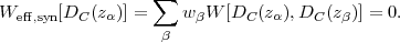(137)

Clearly some of the weights w_β must be negative. This class of techniques assumes nothing about the physics of intrinsic alignments, but because of the extrapolations or negative weights it can amplify observational systematics, and to date it has not been successfully implemented on real data.

A model-dependent alternative, less demanding in terms of observational systematics, is to construct the 3 × 3 symmetric matrix of power spectra of the matter, galaxies, and intrinsic ellipticity,

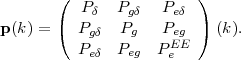(138)

This has six free functions of wavenumber, of which one (P_δ) can be predicted from cosmological parameters. However, since the tidal field is determined by the matter distribution, if galaxy alignments are really determined by the tidal field then they should not additionally care where the other galaxies are: the conditional probability distribution Prob(e|δ, g) = Prob(e|δ). In this case, and in the limit of a Gaussian field, one should have the restriction ⁶⁰

(139)

This relation was assumed by the DETF in their WL parameter forecasts (Albrecht et al. 2006), and if valid it is very useful because it relates the GI contamination (P_eδ) to theory (P_δ), GGL (P_{g δ}), and galaxy-ellipticity correlations at the same redshift (P_eg). Unfortunately, its accuracy is unclear in the nonlinear regime, since for non-Gaussian density fields, Prob(e|δ, g) = Prob(e|δ) no longer implies equation (139); an investigation of this in simulations should be a high priority. Nevertheless, equation (139) may be usable if the GI correlation for late-type galaxies turns out to be far below current upper bounds, in which case even a crude correction could reduce it to below statistical error bars. Further discussions of this approach and an application to observational data may be found in Bernstein (2009), Joachimi and Bridle (2010), and Kirk et al. (2010).

Intrinsic alignments also represent a contaminant to GGL if the "lens" and "source" redshift distributions overlap; some of the "sources" may then be physically associated with the lens and show an alignment that is a result of galaxy formation physics rather than lensing (Bernstein and Norberg 2002, Hirata et al. 2004). However, in this case the availability of good photo-zs solves the problem, since for GGL there are only II alignments, which can be eliminated by restricting cross-correlations to non-overlapping redshift slices. Consistency checks between GGL and cosmic shear may provide a useful route to diagnosing the impact of intrinsic alignments on the latter.

5.6.2. Theoretical uncertainties in the matter power spectrum*

An important systematic error in weak lensing is the prediction of the cosmic shear power spectrum, which — although far more theoretically tractable than galaxy clustering — is not free of uncertainty. WL gets most of its information from the nonlinear regime, where the only way to accurately predict the power spectrum is using large N-body simulations. At the present time, most WL constraints have used physically motivated fitting formulae calibrated to N-body simulations (e.g., Peacock and Dodds 1996, Smith et al. 2003), but these have limited accuracy because of the limited resolution and box size of the simulations and the limited ranges of cosmological parameters that have been explored. The situation has improved dramatically in recent years thanks to Moore's law and the fact that the "interesting" region of parameter space has shrunk considerably. Much improved nonlinear matter power spectrum calculations have been obtained from the "Coyote Universe" simulations (Heitmann et al. 2009, Heitmann et al. 2010, Lawrence et al. 2010). Given this progress, and given that the N-body problem is perfectly well-defined mathematically, we expect that the theoretical uncertainty in the power spectrum for pure dark matter models will not be a limiting systematic for WL.

The situation is more complicated when one goes beyond pure dark matter. Baryons make up ~ 17% of the matter in the universe, and on small scales they do not trace the dark matter. Hydrodynamic simulations can follow them, but one cannot hope to model the processes of cooling, star formation, metal enrichment and feedback from first principles. On quasilinear scales, k ~ few × 0.1h Mpc^-1, the largest uncertainty appears to come from clusters, where redistribution of the radial distribution of baryons affects the 1-halo contribution to the power spectrum. Observations of clusters — in particular measurement of cluster concentrations — may help to constrain this effect (Rudd et al. 2008). It has been proposed to either "self-calibrate" the cluster profile effect (Zentner et al. 2008) or incorporate information from cluster-galaxy lensing (Mandelbaum et al. 2008), although this has not yet been necessary for present cosmic shear experiments.

A second uncertainty is associated with the missing baryon problem — the fact that most of the baryons that should be in galaxy-sized halos (assuming a cosmic baryon:CDM ratio) are not observed in the stellar, H i, and molecular gas components. If these baryons have been ejected from the host halo, e.g. via galactic winds or AGN feedback, then they could reduce the matter power spectrum. These effects were discussed in an idealized "nightmare scenario" by Levine and Gnedin (2006); more recently, the detailed hydrodynamic simulations of van Daalen et al. (2011) have shown a suppression of the matter power spectrum by 1% at k = 0.3 h / Mpc and 10% at k = 1h / Mpc. These effects are large compared to the statistical errors of Stage IV WL experiments. Worrisomely, van Daalen et al. (2011) find that the predictions for the matter power spectrum depend significantly on the treatment of star formation and AGN feedback in the simulations. In their simulations, AGN feedback has the effect of reducing the baryon content of the haloes, consistent with X-ray observations of intrahalo gas: the matter power suppression quoted above is thus within the range of "reasonable" rather than "extreme/unrealistic" models.

Semboloni et al. (2011) show that the results of the simulations can be captured by a parameterized halo model for the baryons, so one may be able to use this approach to marginalize over uncertainties, but at the price of reducing the cosmological information derived from WL measurements on these scales. Moreover, their mitigation procedure involves tuning the halo model to the van Daalen et al. (2011) simulations. Therefore one should worry that the removal of baryonic physics-induced bias seen by Semboloni et al. (2011) might not be realized in practice, if the simulation captures the qualitative features of AGN feedback but does not quantitatively reproduce the correct functional form. Zentner et al. (2012) avoid this issue by fitting cosmic shear power spectra based on the van Daalen et al. (2011) simulations using a mitigation procedure tuned to the Rudd et al. (2008) simulations. However they find that this procedure, while successful on simulated Stage III (DES) survey data, is not adequate for the more ambitious task of Stage IV data analysis.

In summary, it is clear that better predictions for baryonic effects in the matter power spectrum, ancillary observations of baryonic gas to constrain the range of outcomes realized in the real universe, and optimal methods for incorporating these effects with minimal damage to cosmological constraints are critical areas for further investigation.

A final issue is the accuracy of the leading-order mapping from P_δ(k, z) to the shear power spectrum, equation (73). Next-order perturbation theory arguments (Krause and Hirata 2010) suggest that the correction is small, only a few σ for Stage IV experiments. Ultimately, this correction should be computed with ray-tracing simulations that solve the full deflection equation.

5.7. Systematic Errors and their Amelioration: Summary

Summarizing results from our earlier discussion, the principal systematic errors in weak lensing measurements are:

• PSF correction and shape measurement biases (Sections 5.5.2-5.5.5): For the typical case of a PSF of a similar size to the galaxy, the correction of the galaxy ellipticity for PSF effects is of order unity, and the desired accuracy is < 10^-3. This requires both very accurate knowledge of the PSF and appropriate algorithms to correct for it.
• Redshift distribution uncertainties (Section 5.4.3): Using source galaxies at a higher redshift increases the WL power spectrum, and hence there is a degeneracy between z_source and the inferred cosmological parameters. If the source redshift distribution (or distributions, in the case of a tomographic analysis using photometric redshifts) are not well-calibrated, there is a resulting error in the inferred cosmology.
• Intrinsic alignments (Section 5.6.1): The ellipticities of nearby galaxies may be correlated with each other due to formation in a common environment. This "II effect" adds to the observed shear power spectrum and represents a systematic error. There can also be cross-correlation of the intrinsic ellipticity of a nearby galaxy at z = z₁ with the lensing signal on a more distant galaxy at z = z₂ > z₁, since both depend on the tidal field at z = z₁. This latter "GI effect" contaminates all tomographic cross-power spectra and hence is more difficult to remove than II.
• Matter power spectrum uncertainties (Section 5.6.2): Predicting P_m(k, z) from a set of cosmological parameters is a nontrivial task. This can now be done accurately for dark matter only cosmologies (assuming that the dark matter behaves as simple CDM), but on small scales the influence of baryonic physics (cooling, feedback, etc.) is difficult to model.

These errors, and the steps to remove them, are not independent — for example, marginalizing out the intrinsic alignment effects can amplify systematic errors in photometric redshifts (Bridle and King 2007). The development of systematic error budgets and requirements for future surveys thus requires a global analysis of all of the statistical and systematic uncertainties and their possible degeneracies (Bernstein 2009).

We have described numerous strategies for suppressing most of these effects, but a few features stand out. First, exquisite knowledge of the PSF must be achieved through some combination of good engineering (designing a stable telescope and instrument and putting it in the best possible environment), good choice of observing strategy (more dithers and repeat visits), and good algorithms (one needs to generate a homogeneous catalog with well-understood ellipticity errors and selection effects). Second, precise photo-zs over the entire range covered by the survey are desirable for characterizing the redshift distribution, and they are required if one is to even attempt a model-independent removal of intrinsic alignments — something that has not yet successfully been done. To achieve these photo-z requirements, one wants optical and near-IR photometry to distinguish Balmer/4000E breaks from Lyα breaks and spectroscopic samples that span the full range of the WL samples. Cross-correlation against large redshift surveys can be an important tool in photo-z calibration (Newman 2008).

5.8 Advantages of a Space Mission

A space platform offers two critical advantages for weak lensing: (i) the availability of a small and stable PSF, and (ii) the low sky brightness in the near-IR, which allows deeper observations. For this reason, weak lensing has been highlighted as an important science objective for the Euclid and WFIRST space missions.

The small PSF enables the telescope to resolve many more galaxies (see Fig. 17). The space-based PSF size is normally determined by the diffraction limit: for an ideal Airy disk with an unobstructed circular aperture (off-axis telescope), the 50% encircled energy radius EE50 is 0.535 λ / D. This worsens for obstructed telescopes, reaching 1.25 λ/D in the extreme case of blocking 25% of the area of the telescope entrance. Nevertheless, for typical λ (of order 0.8 μm for a visible mission and 1.5 μm for a near-IR mission) and reasonable telescope size (D ≥ 1.1 m) the EE50 radius is several times smaller than the typical ~ 0.3-0.4 arcsec from a good ground-based site. There are additional contributions to the PSF size - charge diffusion, the pixel tophat, aberrations, and pointing jitter - but on a space weak lensing mission these would be designed to be subdominant to diffraction.

A perhaps more important advantage is the stability of the PSF on a space mission, which allows for better characterization. The dominant contribution to a ground-based PSF is from atmospheric turbulence, which varies rapidly as a function of time and field position. This is eliminated in space. Moreover, contributions to the optical distortions from temperature variations and gravity loading can be reduced or (in the latter case) eliminated, particularly at the L2 Lagrange point, in a high Earth orbit during periods where shadow is avoided, and/or by using temperature-controlled optics. The three dominant contributions to PSF ellipticity on a space mission are (i) astigmatism, which causes the ellipticity of the PSF to vary with focus position; (ii) coma from misaligned optics, which at second order leads to ellipticity; and (iii) anisotropic pointing jitter. Of these, (i) and (ii) are functions of mirror positions, whose time and field position dependence are controlled by a small number of parameters. The pointing jitter is the least stable - it may be different in every exposure — but it has a controlled position dependence, no color dependence (at least with all-reflective optics), and can be monitored with the same fine guidance sensors used to point the telescope. Therefore a space mission offers the possibility of a PSF whose entire structure is determined by a small number of parameters that can be tracked as a function of time (Ma et al. 2008). This means it provides the best possibility of providing accurate PSF knowledge at every point in every exposure. The diffraction PSF has the unfortunate feature of having a size that is highly color-dependent (∝ λ / D), and in the presence of aberrations the ellipticity is color-dependent as well. However, in contrast to ground-based observations, the color dependence is controlled by the same wavefront error that determines the PSF morphology.

As already noted, optimal photo-z performance across the entire relevant range of redshifts can be obtained only with continuous coverage from blueward of the 4000 E break (at z = 0) through the near-IR. In particular the Balmer/4000 E feature is always detected except at very high redshift (z > 3), which reduces the number of objects with no breaks identified and provides cleaner separation of the Lyα versus Balmer/4000 E breaks. Collecting photometric data points in the bluer bands (starting at the ~ 3200 E atmospheric cutoff) is quite reasonable from the ground, and in this area there is no major advantage to a space mission. However, as we move to the red the space mission begins to look much more attractive. From the ground, the near-IR sky brightness (relevant for broadband imaging) is dominated by the decay of OH radicals, which are produced in vibrationally excited states at ~ 90 km altitude in the Earth's upper atmosphere (Leinert et al. 1998). The typical sky brightness rises from 18.5 mag AB arcsec^-2 in the Z band through 15.4 mag AB arcsec^-2 in the H band. ⁶¹ In space in the 1-2 μm region the dominant background is instead scattering of sunlight off of interplanetary dust particles (the "zodiacal light"). The typical brightness is ~ 23 mag AB arcsec^-2 near the ecliptic poles and 21.5 mag AB arcsec^-2 in the ecliptic plane (Leinert et al. 1998). Thus in the H band the sky brightness is a factor of 300-1000 lower in space, which means that a space telescope with even ~ 1 m² collecting area would outperform the best ground-based telescopes in terms of near-IR imaging survey speed. Note also that because of the altitude of the OH emitting layer, airplane or balloon based platforms cannot access the low background available in space.

5.9. Prospects

The next several years promise to be very exciting for weak lensing as we enter the Stage III era. Two major wide-field ground-based imagers are coming online in the 2012/13 timeframe: the Dark Energy Camera ⁶² (DECam) at CTIO in the Southern Hemisphere, and the Hyper Suprime Cam (HSC) on Subaru in the Northern Hemisphere (Miyazaki et al. 2006). These will provide great leaps in itendue, roughly 35 m² deg² for DECam and 70 m² deg² for HSC (versus 8 m² deg² for CFHT/MegaCam). The Dark Energy Survey (DES; using DECam) plans to observe 5000 deg² in the grizy bands over five years to ~ 24th magnitude (10σ r band AB, shallower in y). The HSC plans a somewhat deeper and narrower survey, also in grizy (2000 deg², 25th magnitude 10σ). These projects together will measure the shapes of roughly 300 million galaxies and provide accurate photometric redshifts out to z ~ 1.3; this represents a 11/2 order of magnitude increase relative to current data sets. We expect that the use of several revisits and shape measurements in multiple bands, as well as incorporating the lessons from Stage II WL projects such as the CFHTLS and SDSS, will provide additional control over systematic errors in shape measurement. With careful attention to the source redshift distribution as well, and the photo-z capability provided by y-band imaging, the Stage III cosmic shear projects (DES and HSC) should reach the 1% level of precision on the amplitude σ₈, as well as providing high-S / N measurements of its increase as a function of cosmic time. If the stochasticity issue turns out to be tractable, a similar level of precision will be reached by using galaxy-galaxy lensing to constrain the bias of galaxies and infer σ₈ indirectly from galaxy clustering.

The Stage III projects will also mark the completion of the research program of extrapolating the amplitude measured from the CMB forward in time and comparing it to the value of σ₈ measured via WL, and using the agreement of the amplitudes to measure w(z) or test GR. There is a fundamental limitation to this type of comparison coming from reionization: while Planck will measure the CMB power spectrum to very high accuracy, one needs the optical depth τ to convert this into a normalization of the initial perturbations. This seems unlikely to be measured from the CMB E-mode to significantly better than 0.01 due to cosmic variance, foregrounds, and modeling uncertainties (Holder et al. 2003, Mortonson and Hu 2008, Colombo and Pierpaoli 2009). ⁶³

The completion of the DES and HSC will not, however, mark the end of the road for cosmic shear. Because of the reionization degeneracy, the next step will be to make highly accurate measurements of the shape of the signal (dependence on scale and redshift) rather than its amplitude. This is a scientific matter of critical importance: if DES/HSC find a convincing deviation from the expected amplitude of low-redshift structure, one does not know whether this reflects a breakdown of GR at late times (a phenomenon that might be linked to cosmic acceleration) or something that happened to alter the growth of structure between z ~ 10³ and z ~ a few (such as massive neutrinos, though early dark energy would also be a possible explanation). What is needed next is the survey that measures the rate at which the growth of structure is suppressed internally to the low-redshift data. In our Section 8 forecasts we describe deviations from the GR-predicted growth rate using the parameter Δγ (see eqs. 15 and 44), though other choices are possible. Even the Stage III surveys may make only preliminary measurements in this direction. Albrecht et al. (2009) estimated that DES could measure Δγ to a 1σ accuracy of only 0.2 using the evolution of the WL signal, and our fiducial Stage III forecast in Section 8.3 yields σ_Δγ = 0.148 (see Table 9). Clusters calibrated by stacked weak lensing might enable a significantly tighter constraint (Section 8.4, Fig.47), and redshift-space distortions could also enable good measurements of Δγ (Section 7.2). It is not clear, however, that any method will achieve percent-level measurements of the rate of low redshift structure growth in the 2010 decade. Reaching this goal is one of the major drivers for Stage IV projects using WL and other probes of structure growth. It requires highly accurate, low-systematics shape measurements, of galaxies across a wide range of redshifts, including z > 1 where the angular radii of galaxies are small and the shape measurement challenges are immense.

Fortunately, the Stage IV WL experiments are already being planned, although their first light is not expected until ≥2020. There are several approaches. One is the Large Synoptic Survey Telescope (LSST), which would feature a giant-itendue (290 m² deg²) telescope dedicated to optical surveys of the Southern Hemisphere. Over a ten-year operating period, LSST would acquire hundreds of images of every point on the sky, which should go a long way toward identifying and removing any residual sources of PSF systematics. The incorporation of 6 bands (ugrizy) will likely lead to the best photometric redshifts practical from the ground over such a wide area. LSST will survey the entire extragalactic sky available from the south, perhaps 12,000-15,000 deg². The usable density of source galaxies, particularly at high redshift, is not certain as it depends on both advances in measuring galaxies small compared to the PSF and the quality of photometric redshifts in the notorious 1.3 < z < 2 range. However, by achieving high S/N on almost every resolved galaxy, LSST is likely to represent the "ultimate experiment" for ground-based optical weak lensing.

An alternative approach is to exploit the small and stable PSF and availability of the near-IR bands from space, as planned for ESA's Euclid mission (scheduled launch in 2020) and the NASA WFIRST mission (launch date to be determined; see below). Euclid will be a 1.2 m telescope with a 0.5 deg² focal plane that will survey 15,000 deg² in a parallel WL+BAO mode, with shape measurements performed in a broad red band (0.55-0.92 μm). Euclid will have only 3-4 observations of each galaxy, but this is predicted to be acceptable given the much greater stability of Euclid's PSF relative to anything possible on the ground. At ~ 30 galaxies per arcmin², Euclid would measure shapes for ~ 1.6 billion galaxies. Euclid will also obtain near-IR photometry in three bands, which will be combined with ground-based optical photometry (from LSST where available) for photometric redshifts; the IR imaging is underresolved and will not be used for shape measurements. WFIRST, in the "DRM1" configuration described by Green et al. (2012), would be a 1.3 m, unobstructed (i.e., off-axis secondary) infrared space telescope capable of surveying 1400 deg² / yr in a combined WL+BAO mode (4-band imaging and slitless spectroscopy with resolution λ/Δλ ≈ 600). The baseline WL program has 5-8 exposures in each of three shape measurement filters (J, H, and K), with an effective source density n_eff = 40 arcmin^-2, and in a shorter wavelength filter (Y) that provides additional information for photometric redshifts. (LSST or other ground-based data are again required to provide optical photometry.) Multiple bands provide control of color-dependence of the PSF, and the degree of data redundancy is much higher than in Euclid because of the larger number of exposures and the ability to correlate shape measurements in different bands — the WL signal should be achromatic, but many systematics would not be. However, this greater redundancy, and the fact that the telescope is shared with other science programs, comes at the expense of what will likely be a smaller survey. The Green et al. (2012) design reference mission calls for 2.4 years of high-latitude imaging and spectroscopy (out of a 5-year mission lifetime), which is sufficient to cover 3400 deg². ⁶⁴ As mentioned in Section 1.3, the transfer of two 2.4-m on-axis space telescopes from the U.S. National Reconnaissance Office (NRO) to NASA opens an alternative route to WFIRST, with initial ideas described by Dressler et al. (2012). While this implementation may not increase the survey area ⁶⁵, the superior angular resolution and light-gathering power of this hardware make it the only plausible option (at least in the optical-NIR bands) to reach source galaxy densities of ~ 70 galaxies/arcmin² over thousands of deg². A detailed study of a 2.4-m implementation of WFIRST is ongoing, with a report planned for April 2013.

By the end of the 2020s, we should have a rich data set from all three of these projects (LSST, Euclid, and WFIRST) — and perhaps also from a large-scale radio interferometer such as the SKA. These surveys represent very different approaches to the Stage IV WL problem and will provide for multiple cross-checks of final results and internal cross-correlations of different data sets. The total number of galaxies with accurately measured shapes will probably reach ~ 4 billion, with most observed by at least two instruments and some with all three. Robust measurements of the suppression of the growth of structure to σ_Δγ ≈ 0.03 — a factor of several better than Stage III — should then be possible (see Table 8), as well as tests of other possible deviations from ΛCDM that we have not yet imagined. But a great deal of work will be necessary before then to ensure that the systematic errors are controlled at this level.

For our forecasts in Section 8 we adopt a fiducial Stage IV WL program that assumes an effective source density n_eff = 23 arcmin^-2 over 10⁴ deg², for a total of 8.3 × 10⁸ shape measurements in 14 bins of photometric redshift (see Section 8.1 for details). We incorporate (and marginalize over) a multiplicative shear calibration uncertainty of 2 × 10^-3 and a mean photo-z uncertainty of 2 × 10^-3; these are aggregate values, and are larger by √14 in each photo-z bin. LSST and Euclid both anticipate a larger number of shape measurements and thus smaller statistical errors than our fiducial program. The baseline WFIRST DRM1 survey has a factor of two fewer shape measurements, but the mission's technical requirement for shape systematics is a factor of two better. Thus, our fiducial program is conservative relative to the stated goals of all three experiments, though highly ambitious relative to the current state of the field.

For this fiducial Stage IV program, Figure 19 shows the predicted shear power spectrum and 1σ statistical errors, in each of the 14 photo-z bins. In addition to these auto-spectra, the data allow measurements of N_bin(N_bin - 1) cross-spectra among the bins, providing additional statistical power and tests for intrinsic alignment and other systematics. In a given photo-z bin, the errors in different l bins are independent. However, the errors from one photo-z bin to another are correlated because the same foreground structure can lens galaxies in multiple background redshift shells. We compare the statistical errors to the impact of cosmological parameter changes in Section 8.7. The aggregate statistical precision on the overall amplitude of the WL power spectrum, i.e., on a constant multiplicative factor applied to the auto- and cross-correlations in all photo-z bins, is ≈ 0.21%. The corresponding error on σ₈, treated as a single parameter change, is about three times smaller because the power spectrum scales as σ₈³ in the regime where it is best measured. The right panel compares the statistical errors in four representative photo-z bins to the effects of a multiplicative shear calibration bias of 2 × 10^-3, a mean photo-z bias of 2 × 10^-3, or an additive shear bias of 3 × 10^-4. We see that systematic errors of this magnitude would be smaller than the statistical errors in an individual photo-z bin, but the overall impact would be larger than the aggregate statistical errors. Thus, for our fiducial assumptions the Stage IV program is systematics limited rather than statistics limited, but not by an enormous factor. Even though our assumptions for this fiducial program are arguably conservative, it would achieve powerful constraints on the cosmic expansion history and the history of structure growth, as discussed in Section 8.

Figure 19. (Left) The predicted cosmic shear power spectrum and statistical errors in each of 14 photo-z bins assuming a ΛCDM cosmological model with the parameters of Albrecht et al. (2009) and the survey parameters of our fiducial Stage IV WL program. (Right) Impact of systematic errors relative to statistical errors. For three of the photo-z bins from the left panel, error bars show the ± 1σ statistical errors (in bins of width Δlogl = 0.2 dex), with vertical offsets between bins for clarity. Solid, dashed, and dotted curves show, respectively, the effect of a multiplicative shear calibration bias of 2 × 10-3 × √14 (orange), a mean photo-z offset of 2 × 10-3 × √14 (green), or an additive shear bias of 3 × 10-4 × √14 (blue) per z-bin. (The √14 is inserted here since an actual survey would combine all 14 bins.) The power in the additive shear bias was equally distributed in lnl for the purposes of this plot.

Is there a future for WL beyond Stage IV, both in terms of science motivation and technical capability? It seems unlikely that there would be a follow-on experiment that consists of simply a super-size LSST, Euclid, or WFIRST, particularly given that these experiments will come within a factor of a few of the cosmic variance limit at several tens of galaxies per arcmin². Rather the more distant future would have to involve new technology and a new science case not subject to the usual limitations. An example might be to look for lensing by primordial gravitational waves, which is not practical using galaxies as sources (Dodelson et al. 2003) but is at least in principle possible using highly-redshifted 21 cm radiation as the source, even for tensor-to-scalar ratios as low as 10^-9 (Book et al. 2012). But we have now entered the speculative realm of post-2030 science and technology, where our ability to forecast the future is of limited reliability. We thus conclude our discussion of weak lensing here.

²⁸ Warning: these scalings are altered even at modest redshift, or in the nonlinear regime where the exponent of σ₈ becomes closer to 3. Back.

²⁹ The cosmography distance scale suffers from three degeneracies, including the absolute-scale degeneracy that affects supernova measurements; see Section 5.2.7. Back.

³⁰ These approximations are sufficient to analyze present power spectrum data, but corrections to (iv) will become necessary in the future. Back.

³¹ The derivation of equation (57) can be found in many works, though not always in the same notation. See, e.g., eq. (6.9) in the classic review by Bartelmann and Schneider (2001). The appendix of Hirata and Seljak (2003a) gives a shorter derivation in more similar notation. Back.

³² As discussed further in Section 5.5.2 below, a typical population of optically imaged galaxies (bulges and randomly oriented disks) has an rms ellipticity e_rms ~ 0.4 per component, which translates into an rms shear error σ_γ ≈ 0.2 via the shear response factor (eq. 112). Because there are two components to shear one might expect to do a factor of √2 better in statistical measurements, but in the shear correlation function or power spectrum only one of the two measurable components (the "E-mode" discussed in the next section) contains a cosmological signal at leading order, so the relevant number for order-of-magnitude sensitivity estimates is generally σ_γ ≈ 0.2. Similarly, for galaxy-galaxy or cluster-galaxy weak lensing, only the tangential shear contains cosmological information. Back.

³³ See Limber (1953) and Limber (1954) for an introduction to the theory. An exposition in terms of the power spectrum is given by Peebles (1973). Back.

³⁴ Warning: many conventions in use! Back.

³⁵ The Heaviside step function Θ is technically unnecessary in equation (74), but it is convenient when considering multiple populations of sources. Back.

³⁶ The leading order curved sky correction is the replacement of the scalar wavenumber |l| with [l(l + 1)]^1/2, where here "l" is the spherical multipole number. Further corrections are of the order of 1/l² and are most important for the lowest multipoles. Back.

³⁷ There is also a factor of Ω_m H₀² in the window functions, but for now we will assume this combination has been measured accurately from the CMB. Our forecasts in Section 8 marginalize over the uncertainty in this combination, which matters at the precision of Stage IV experiments. Back.

³⁸ This is the same reason that the "∞" setting on the focus knob for a camera is not special. Back.

³⁹ The EEB and BBB bispectra flip sign under reflections of the triangle, and some convention, e.g. that the sides are given in counterclockwise order, must be imposed to avoid ambiguity. Back.

⁴⁰ Equivalent to ~ ω² h, where ω is the gravitational wave frequency and h is the strain. Back.

⁴¹ The premier lensing instrument on the HST (the Advanced Camera for Surveys) failed in January 2007. While its wide-field channel was restored during the 2009 servicing mission, the sky coverage possible with ACS is not competitive with next-generation ground-based surveys, and it seems unlikely a major cosmic shear program will be undertaken with HST. Rather, the next major steps in space-based cosmic shear will likely be the Euclid mission planned for 2020 and the WFIRST mission planned for the early 2020s. Back.

⁴² Since lensing measures δρ rather than δρ / ρ, there is a factor of Ω_m in this measurement. Back.

⁴³ A re-analysis with the final SDSS imaging data set and improved treatment of the stochasticity is underway. Back.

⁴⁴ By "optical," we mean to include near-infrared wavelengths λ > 0.7 μm at which stars are still the dominant source of luminosity, and which are observed through traditional optical telescopes and with detector technology based on the creation of electron-hole pairs in semiconductors. Back.

⁴⁵ We give the E-mode noise here. There is an equal amount of shape noise power in the B-mode, but the lensing B-mode is used only as a systematics test because it contains no cosmological signal to first order. Back.

⁴⁶ High-amplitude features such as clusters may still be visible. Back.

⁴⁷ In practice the Galactic Plane must be avoided, so it is unlikely that optical astronomy would push beyond f_sky ~ 0.7 for any cosmological application. Back.

⁴⁸ For realistic non-Gaussian profiles, the shape measurement error is usually worse by of order 20%. Back.

⁴⁹ Primordial gravitational waves can generate a B-mode on large scales, but such gravitational waves are adiabatically damped on angular scales below a degree. Thus the ~ 10'-scale B-mode should be dominated by lensing. Back.

⁵⁰ Massey et al. (2007a) Section 3.1.1 give an excellent technical review of the methods derived from KSB. Back.

⁵¹ Here we use the term "PSF" to include not just the image of a point source produced by the telescope optics but also pointing jitter and detector effects. For example, if the detector has square pixels, the PSF is that delivered by the telescope convolved with a square top-hat function. Back.

⁵² It is important to recall that the definition of oversampling required for equation (106) operates in Fourier space. The commonly used condition for oversampling that the FWHM should exceed 2 pixels is a good rule of thumb for smooth profiles such a Gaussian, but it is not appropriate for general PSFs. Back.

⁵³ Much of the HST / COSMOS weak lensing work used the "Drizzle" algorithm (Fruchter and Hook 2002), which in general leads to a slightly different PSF in each pixel. However, this did not represent a limiting systematic for the ~ 2 deg² observed in COSMOS. Back.

⁵⁴ This is easily seen because the measure d²x in equation (113) is shear-invariant. Back.

⁵⁵ See also Kaiser (2000), which contains many of these ideas but seems to have been promptly forgotten by most of the WL comminity! Back.

⁵⁶ Note that W must transform as a vector under rotations, and W_e as a spin-2 tensor. Back.

⁵⁷ As a reminder, here x is used to refer to the location within the image of each star, i.e., of order ~ 1", whereas the independent variable θ accounts for variation across the entire field, of order ~ 1°. Back.

⁵⁸ If one interprets the model of equation (134) as applying to the unweighted ellipticity field, then converting to a galaxy-weighted field introduces a B-mode. However it is much smaller than the E-mode signal and vanishes in the linear regime. Back.

⁵⁹ This has been measured as the line-of-sight integral of the correlation function, w(r_p) where r_p is the transverse separation, which contains the same information as the power spectrum. Back.

⁶⁰ This is a slightly more general relation than assuming that the galaxies are linearly biased with no stochasticity, in which case one could replace P_δ(k) / P_{g δ}(k) → 1/b. Back.

⁶¹ See the WFCAM website, http://casu.ast.cam.ac.uk/surveys-projects/wfcam, and beware of Vega to AB conversions, which are significant in the near-IR. Back.

⁶² http://www.darkenergysurvey.org/ Back.

⁶³ In the more distant future, 21 cm measurements may improve our understanding of reionization to the point where this limitation is removed; however such an advanced understanding is not anticipated in the immediate future. Back.

⁶⁴ An additional 0.45 years would be devoted to an imaging and spectroscopic survey for supernovae. Back.

⁶⁵ In wide-field ground-based surveys, an increase in telescope aperture, e.g. 2 m → 4 m, increases the itendue, resulting in a faster survey at the same seeing-limited resolution. For space-based surveys, the natural choice when receiving a larger telescope is to maintain the same sampling of the PSF (and hence the same f-ratio if the detector properties remain fixed), which results in each pixel subtending a smaller number of arcseconds. The itendue and hence survey speed to reach the same extended-source sensitivity are unchanged if the pixel count is held fixed, but the angular resolution is improved as ~ λ / D. This is of course an enormous advantage for weak lensing. Back.