


In the following we describe the evolution and nucleosynthesis for representative low- and intermediate-mass stars. All have a metallicity Z = 0.02 1. According to the most recent solar abundances from Asplund et al. (2009) the global solar metallicity is Z = 0.0142, which makes these models slightly super solar, with a [Fe/H] = + 0.14 2.
To illustrate the evolution of low- and intermediate-mass stars we use new stellar evolutionary sequences with masses between 1 and 8 M⊙ and Z = 0.02 calculated with the same version of the Mt Stromlo/Monash Stellar Structure code described in Kamath et al. (2012). Within this grid of models, the divide between low-mass stellar evolution and intermediate is at about 2 M⊙, as we discuss below. These models will also introduce the basic principles of the evolution of all stars that evolve up to the AGB. The theoretical evolutionary tracks for a sample of these models are shown in Figure 2 and include all evolutionary phases from the zero age main sequence through to the AGB.
All stars begin their nuclear-burning life on the main sequence, where fusion converts H to He in the stellar core. The majority of a star’s nuclear-burning life is spent on the main sequence, which is why most stars in the night sky and most stars in a typical colour-magnitude diagram are in this phase of stellar evolution.
The 1 M⊙ model in Figure 2 burns H on the main sequence via the pp chains. In contrast, the models with M ≥ 2 M⊙ shown in Figure 2 mostly burn H in the core via CNO cycling. The higher temperature dependence of the CNO cycles, with a rate roughly ∝T16 − 20 (compared to a rate approximately ∝T4 for the pp chains at Z = 0.02), produces a steep energy generation rate and results in the formation of a convective core. It is convenient to divide the zero-age main sequence (ZAMS) into an ‘upper’ and ‘lower’ main sequence, which is reflected in slightly different mass-radius and mass-luminosity relationships for these two regions. The division between the two is instructive: stars on the lower main sequence have convective envelopes, radiative cores, and are primarily powered by the pp chains. Conversely, stars on the upper main sequence show radiative envelopes, convective cores, and are powered primarily through the CN (and ON) cycles. The dividing mass between the upper and lower main sequence is at about 1.2 M⊙ for Z = 0.02.
The larger a star’s mass the larger is its gravity. Hence it requires a substantial pressure gradient to maintain hydrostatic equilibrium. The central pressure is therefore higher and in turn so is the temperature. This means that more massive stars burn at much higher luminosities and given that fusing four protons into one 4He nucleus produces a constant amount of energy, then the duration of the H burning phase must be correspondingly lower as the stellar mass increases. From a quick inspection of Figure 2 it is clear that the 6 M⊙ model is much brighter on the main sequence than the 2 M⊙ model by almost two orders of magnitude. Core H exhaustion takes place after approximately 1 × 10⁹ years (or 1 Gyr) for the 2 M⊙ model but only 53 million years for the 6 M⊙ model.
Following core H exhaustion the core contracts and the star crosses the Hertzsprung Gap. Nuclear burning is now established in a shell surrounding the contracting 4He core. Simultaneously, the outer layers expand and cool and as a consequence become convective, due to an increase in the opacity at lower temperatures. The star runs up against the Hayashi limit, where the coolest envelope solution corresponds to complete convection. The star cannot cool further and it begins its rise up the giant branch while the convective envelope grows deeper and deeper (in mass). This is shown in Figure 3 for the 1 M⊙ model. This deepening of the convective envelope leads to mixing of the outer envelope with regions that have experienced some nuclear processing, with the result that the products of H burning are mixed to the surface. This is called the ‘first dredge-up’, hereafter FDU.
 |
Figure 3. First dredge-up in the 1 M⊙, Z = 0.02 model. The left panel shows the HR diagram and the right panel shows the luminosity as a function of the mass position of the inner edge of the convective envelope. We can clearly see that the envelope begins to deepen just as the star leaves the main sequence, and reaches its deepest extent on the RGB, marking the end of FDU. Further evolution sees the star reverse its evolution and descend the RGB briefly before resuming the climb. This corresponds to the observed bump in the luminosity function of stellar clusters (see text for details). |
The star is now very big (up to ~ 100 times its radius on the main sequence) but most of the mass in the core is within a small fraction of the total radius. A consequence of this is that the outer layers are only tenuously held onto the star and can be lost through an outflow of gas called a stellar wind. At present we do not know how much mass is lost during the ascent of the RGB. This may be perhaps as much as 30% of the star's total mass for the lowest mass stars that spend the longest time on the RGB. Kepler data for metal-rich old open clusters have provided some constraints, with the amount of mass lost on the RGB estimated to be less than results from applying the commonly used Reimer's mass-loss prescription (Reimers 1975; Kudritzki & Reimers 1978; Miglio et al. 2012). While there are refinements to the Reimer’s mass-loss law (Catelan 2000; Schröder & Cuntz 2005, 2007) we are still lacking a detailed understanding of the physical mechanism responsible for mass loss on the RGB.
During the ascent of the RGB our low- and intermediate-mass stars experience the FDU, which we will address in detail in Section 2.2. Simultaneously, the He core continues to contract and heat and in the case of low-mass stars becomes electron degenerate. Neutrino energy losses become important, and since they are highly dependent on density, they dominate in the centre. This produces a cooling and can cause the mass location of the temperature maximum to move outward. The RGB lifetime is terminated when the necessary temperatures for central He ignition are reached, at about 100 million K. For our low-mass stars the triple alpha reactions are ignited at the point of maximum temperature and under degenerate conditions (Despain 1981; Deupree 1984).
The electron degenerate equation of state results in the temperature and density being essentially decoupled. When He does begin to fuse into C, the energy released does not go into expansion but stays as thermal energy, raising the temperature of the plasma locally. This leads to a much higher burning rate and a runaway result, leading to a violent and explosive He ignition that is known as the ‘core He flash’.
The maximum initial mass for the core He-flash to occur is about 2.1 M⊙ at Z = 0.02 using the new grid of models presented here, which include no convective overshoot (similar to the models of Karakas, Lattanzio, & Pols 2002, where the maximum mass is at about 2.25 M⊙). This is the dividing line between low- and intermediate-mass stars. In contrast, models which include overshooting from the convective H-burning core find that this division occurs at a lower mass of M ≈ 1.6 M⊙ (Bertelli et al. 1986a).
For intermediate-mass stars, the cores are not degenerate and He is ignited under quiescent conditions. These stars often do not proceed as far up the RGB as do low-mass stars, prior to He ignition. As a consequence their RGB phase is shorter and the FDU phase can be terminated relatively early for these more massive stars. This has consequences for colour-magnitude diagrams and is demonstrated in Figure 2. For example, the 2 M⊙ model has a long RGB lifetime of ≈ 200 × 106 years or 200 Myr. This means that while the minimum effective temperature attained by the 2 M⊙ red-giant model is less (Teff ≈ 3 600 K) than the 6 M⊙ model (Teff ≈ 4 100 K), the peak RGB luminosity is similar, at log 10(L / L⊙) ≈ 3.2. This means that old low-mass RGB populations are observable out to great distances (e.g., Galactic GCs and dwarf spheroidal galaxies, which are dominated by old low-mass stars). Note the contrast to the 3 M⊙ model, which has a peak RGB luminosity that is more than 10 times lower, at only 140 L⊙ (due to ignition of He under non-degenerate conditions).
Following core He ignition the star settles down to a period of central He burning, where He burns in a convective core and H in a shell, which provides most of the luminosity. The Coulomb repulsion is larger for He than for H and more particle (kinetic) energy is required to sustain the triple-alpha process. This then requires that the temperature is higher for He burning. Note also that about a factor of 10 less energy is produced by the triple alpha process per gram of fuel than during H burning. The overall result is the core He burning phase is shorter than the main sequence. For example, for the 2 M⊙ model core He burning lasts 124 Myr (a figure of about 100 Myr is typical for low-mass stars), compared to ≈ 13 Myrs for the 6 M⊙ model. Helium burning increases the content of 12C, which in turn increases the abundance of 16O from the reaction 12C(α, γ)16O.
The details of He burning are subject to uncertainties that are all too often ignored or dismissed. We have known for decades that the fusion of He into C and O produces a discontinuity in the opacity at the edge of the convective core (Castellani, Giannone, & Renzini 1971a). This means that there is an acceleration at the edge of the core. In other words there is no neutrally stable point which would be the edge of the core if one were using the Schwarzschild or Ledoux criterion for determining the borders of convective regions. The result is that the convective core grows with time. The next complication is that the variation of temperature and density is such that there is a local minimum in the radiative gradient in the convective region and this causes the region to split into a convective core and a ‘semi-convective’ region (Castellani, Giannone, & Renzini 1971b).
This semi-convection extends the duration of the core He burning phase by mixing more fuel into the core. Star counts in clusters clearly show that observations require this extension to the core He burning phase, and models constructed without semi-convection are a poor match (Buzzoni et al. 1983; Buonanno, Corsi, & Fusi Pecci 1985).
There is yet another complication that arises as the star approaches the exhaustion of its core He supply. Theoretical models show that as the He content decreases, the convective core is unstable to rapid growth into the semi-convective region. This results in ‘breathing pulses’ of the convective core (Gingold 1976; Castellani et al. 1985). These mix more He into the core and further extend the lifetime in this phase. While this behaviour shows many of the signs of a numerical instability, an analytic study by Sweigart & Demarque (1973) showed that there is a genuine physical basis for the instability, and indeed verified that it should only occur when the central He mass fraction reduces below about 0.12. Nevertheless, appealing again to star counts as a proxy for timescales, the data seem to argue against the reality of these pulses (Renzini & Fusi Pecci 1988; Caputo et al. 1989, but see also Campbell et al. 2013).
This leaves us in the most unsatisfactory position. We have an instability shown by models, which theory can explain and indeed argues to be real, but that the data do not support. Further, we have no obvious way to calculate through this phase in a way that removes the breathing pulses (although see Dorman & Rood 1993). What is worse is that the details of the evolution through this phase determine the size of the He exhausted core and the position of the H-burning shell as the star arrives on the early AGB. The star must now rapidly adopt the structure of a thermally-pulsing AGB star, by which we mean that burning shells will burn through the fuel profile resulting from the earlier evolution until they reach the thermally-pulsing AGB structure. This results in removing some of the uncertainty in the structure that exists at the end of core He burning. But it is still true that the subsequent evolution on the AGB is critically dependent on the core size which is poorly understood because of uncertainties during the prior core He burning phase.
Following exhaustion of the core He supply, low- and intermediate-mass stars proceed toward the red giant branch, now called the ‘asymptotic giant branch’ because the colour-magnitude diagrams of old clusters show this population seemingly joining the first giant branch almost asymptotically. A better name may have been the less commonly used ‘second giant branch’, but AGB is now well establi-shed.
For stars more massive than about 4 M⊙ (depending on the composition) or with H-exhausted core masses ≳ 0.8 M⊙ the convective envelope extends quite some distance into the H-exhausted region. It usually reaches deeper than during the FDU (e.g., Boothroyd & Sackmann 1999). This event is called the ‘second dredge-up’, hereafter SDU. In both cases (FDU and SDU) we are mixing to the surface the products of H burning, so qualitatively the changes are similar. However, there are substantial quantitative differences, as we discuss below in Section 2.2.
We have outlined the evolution of low- and intermediate-mass stars above. Now we look in more detail at the first and second dredge-up prior to the thermally-pulsing AGB. Figure 4 shows the different dredge-up processes that stars experience as a function of their mass. It also shows the rough qualitative changes in surface abundances that result.
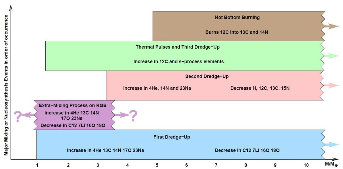 |
Figure 4. A schematic diagram showing the mass dependence of the different dredge-up, mixing, and nucleosynthesis events. The species most affected are also indicated. The lower mass limits for the onset of the SDU, third dredge up, and HBB depend on metallicity and we show approximate values for Z = 0.02. Note that the ‘extra-mixing’ band has a very uncertain upper mass-limit, because the mechanism of the mixing is at present unknown. |
2.2.1. Abundance changes due to FDU
The material mixed to the envelope by the FDU has been subjected to partial H burning, which means it is still mostly H but with some added 4He and the products of CN cycling. Figure 5 shows the situation for a 2 M⊙ model. The upper panel shows the abundance profile after the star has departed the main sequence and prior to the FDU. We have plotted the major species and some selected species involved in the CNO cycles. The lower panel is taken at the time of the maximum depth of the convective envelope. The timescale for convective mixing is much shorter than the evolution timescale so mixing essentially homogenises the region instantly, as far as we are concerned.
 |
Figure 5. Composition profiles from the 2 M⊙, Z = 0.02 model. The top panel illustrates the interior composition after the main sequence and before the FDU takes place, showing mostly CNO isotopes. The lower panel shows the composition at the deepest extent of the FDU (0.31 M⊙), where the shaded region is the convective envelope. Surface abundance changes after the FDU include: a reduction in the C/O ratio from 0.50 to 0.33, in the 12C / 13C ratio from 86.5 to 20.5, an increase in the isotopic ratio of 14N / 15N from 472 to 2 188, a decrease in 16O / 17O from 2 765 to 266, and an increase in 16O / 18O from 524 to 740. Elemental abundances also change: [C/Fe] decreases by about 0.20, [N/Fe] increases by about 0.4, and [Na/Fe] increases by about 0.1. The helium abundance increases by ΔY ≈ 0.012. |
Typical surface abundance changes from FDU are an increase in the 4He abundance by ΔY ≈ 0.03 (in mass fraction), a decrease in the 12C abundance by about 30%, and an increase in the 14N and 13C abundances. In Table 1 we provide the predicted post-FDU and SDU values for model stars with masses between 1 and 8 M⊙ at Z = 0.02. We include the He mass fraction, Y, the isotopic ratios of C, N, and O, and the mass fraction of Na.
| Mass | Event | Y | C/O | 12C/13C | 14N/15N | 16O/17O | 16O/18O | X(23Na) |
| Initial | 0.280 | 0.506 | 86.50 | 472 | 2765 | 524 | 3.904(-5) | |
| 1.00 | FDU | 0.304 | 0.449 | 28.26 | 884 | 2720 | 556 | 3.904(-5) |
| SDU | 0.304 | 0.445 | 26.75 | 931 | 2617 | 560 | 3.911(-5) | |
| 1.30 | FDU | 0.303 | 0.392 | 24.07 | 1362 | 1989 | 627 | 3.941(-5) |
| SDU | 0.303 | 0.390 | 23.43 | 1395 | 1977 | 629 | 3.942(-5) | |
| 1.50 | FDU | 0.300 | 0.362 | 22.31 | 1688 | 930.6 | 674 | 4.157(-5) |
| SDU | 0.300 | 0.360 | 21.74 | 1736 | 913.8 | 678 | 4.165(-5) | |
| 1.90 | FDU | 0.292 | 0.343 | 21.46 | 1948 | 374.6 | 710 | 4.630(-5) |
| SDU | 0.292 | 0.341 | 21.03 | 1994 | 372.2 | 714 | 4.638(-5) | |
| 2.00 | FDU | 0.292 | 0.326 | 20.49 | 2188 | 265.8 | 741 | 4.840(-5) |
| SDU | 0.292 | 0.325 | 20.16 | 2224 | 265.2 | 743 | 4.844(-5) | |
| 2.25 | FDU | 0.291 | 0.320 | 20.15 | 2368 | 214.6 | 754 | 5.112(-5) |
| SDU | 0.291 | 0.320 | 20.00 | 2385 | 214.4 | 754 | 5.114(-5) | |
| 2.50 | FDU | 0.294 | 0.320 | 19.89 | 2610 | 240.0 | 754 | 5.358(-5) |
| SDU | 0.294 | 0.319 | 19.73 | 2633 | 239.4 | 756 | 5.363(-5) | |
| 3.00 | FDU | 0.300 | 0.322 | 19.57 | 2912 | 301.3 | 751 | 5.643(-5) |
| SDU | 0.300 | 0.319 | 19.30 | 2970 | 294.7 | 755 | 5.666(-5) | |
| 3.50 | FDU | 0.298 | 0.323 | 19.43 | 2950 | 327.1 | 748 | 5.683(-5) |
| SDU | 0.298 | 0.319 | 19.08 | 3051 | 309.1 | 756 | 5.752(-5) | |
| 4.00 | FDU | 0.293 | 0.332 | 19.56 | 2780 | 441.6 | 728 | 5.469(-5) |
| SDU | 0.293 | 0.328 | 19.17 | 2892 | 415.6 | 737 | 5.553(-5) | |
| 4.50 | FDU | 0.293 | 0.325 | 19.18 | 2912 | 377.8 | 743 | 5.603(-5) |
| SDU | 0.297 | 0.320 | 18.65 | 3147 | 357.9 | 755 | 5.791(-5) | |
| 5.00 | FDU | 0.291 | 0.324 | 19.06 | 2886 | 375.5 | 745 | 5.567(-5) |
| SDU | 0.309 | 0.322 | 18.74 | 3289 | 367.5 | 751 | 5.962(-5) | |
| 5.50 | FDU | 0.289 | 0.324 | 18.98 | 2843 | 381.8 | 746 | 5.510(-5) |
| SDU | 0.322 | 0.325 | 18.68 | 3542 | 379.3 | 747 | 6.223(-5) | |
| 6.00 | FDU | 0.289 | 0.324 | 18.90 | 2870 | 384.5 | 746 | 5.529(-5) |
| SDU | 0.333 | 0.325 | 18.60 | 3798 | 381.5 | 747 | 6.472(-5) | |
| 7.00 | FDU | 0.291 | 0.324 | 18.68 | 3035 | 397.4 | 748 | 5.665(-5) |
| SDU | 0.350 | 0.325 | 18.40 | 4275 | 395.4 | 750 | 6.885(-5) | |
| 8.00 | FDU | 0.296 | 0.324 | 18.47 | 3281 | 406.9 | 750 | 5.881(-5) |
| SDU | 0.362 | 0.325 | 18.21 | 4675 | 406.4 | 637 | 7.205(-5) | |
The C isotopic ratio is a very useful tracer of stellar evolution and nucleosynthesis in low- and intermediate-mass stars. First, this is because the 12C / 13C ratio is one of the few isotopic ratios that can be readily derived from stellar spectra which means that there are large samples of stars for comparison to theoretical calculations (e.g., Gilroy & Brown 1991; Gratton et al. 2000; Smiljanic et al. 2009; Mikolaitis et al. 2010; Tautvaišienė et al. 2013). Second, the C isotope ratio is predicted to vary significantly at the surface as a result of the FDU (and SDU) as shown in Figure 6 and in Table 1. This figure shows that the number ratio of 12C / 13C drops from its initial value (typically about 89 for the Sun) to lie between 18 and 26 (see also Charbonnel 1994; Boothroyd & Sackmann 1999). Comparisons for intermediate-mass stars are in relatively good agreement with the observations, to within ~ 25% (El Eid 1994; Charbonnel 1994; Boothroyd & Sackmann 1999; Santrich, Pereira, & Drake 2013). But the agreement found at low luminosities is not seen further up the RGB (e.g., Charbonnel 1995), as discussed in Section 2.2.4.
 |
Figure 6. Surface abundance predictions from Z = 0.02 models showing the ratio (by number) of 12C / 13C, 14N / 15N, and 16O / 17O after the first dredge-up (red solid line) and second dredge-up (blue dotted line). |
In Figure 7 we show the innermost mass layer reached by the convective envelope during FDU (solid lines) and SDU (dashed lines) as a function of the initial stellar mass and metallicity. The deepest FDU occurs in the Z = 0.02 models at approximately 2.5 M⊙ with a strong metallicity dependence for models with masses over about 3 M⊙ (Boothroyd & Sackmann 1999). In contrast there is little difference in the depth of the second dredge-up for models with ≳ 3.5 M⊙ regardless of metallicity. In even lower metallicity intermediate-mass stars, the RGB phase is skipped altogether because core He burning is ignited before the model star reaches the RGB so that the first change to the surface composition is actually due to the second dredge-up.
 |
Figure 7. Innermost mass layer reached by the convective envelope during the first dredge-up (solid lines) and second dredge-up (dashed lines) as a function of the initial stellar mass and metallicity. The mass co-ordinate on the y-axis is given as a fraction of the total stellar mass (Mdu / M0)—from Karakas (2003). |
One check on the models concerns the predictions for O isotopes. Broadly, the CNO cycles produce 17O but significantly destroy 18O, with the result that the FDU should increase the observed ratio of 17O / 16O and decrease the observed ratio of 18O / 16O (e.g., Table 1 and Dearborn 1992). Spectroscopic data, where available, seem to agree reasonably well with the FDU predictions (Dearborn 1992; Boothroyd, Sackmann, & Wasserburg 1994), but see also Section 2.2.4.
The effect of the first dredge-up on other elements (besides lithium, which we discuss in Section 2.4 below) is relatively minor. It is worth noting that there is some dispute about the status of sodium. Figure 8 shows that sodium is not predicted to be significantly enhanced in low-mass stars by the FDU or by extra-mixing processes (Charbonnel & Lagarde 2010) at disk metallicities. This agrees with El Eid & Champagne (1995) who find modest enhancements in low mass (0.1 dex) and intermediate mass (0.2 - 0.3 dex) stars. Observations are in general agreement with models with masses ≳ 2 M⊙, where enhancements of up to [Na/Fe] ≲ 0.3 are found in stars up to 8 M⊙ at Z = 0.02 (Figure 8). This result is confirmed by observations that show only mild enhancements of [Na/Fe] ≲ +0.2 (Hamdani et al. 2000; Smiljanic et al. 2009). But this is in contradiction with other studies showing typical overabundances of + 0.5 (Bragaglia et al. 2001; Jacobson, Friel, & Pilachowski 2007; Schuler, King, & The 2009). The reasons for the conflicting results are not well understood; we refer to Smiljanic (2012) for a detailed discussion of observational uncertainties.
 |
Figure 8. Predicted [Na/Fe] after the FDU and SDU for the Z = 0.02 models. |
Theoretical models must confront observations for us to verify that they are reliable or identify where they need improvements. In the current context there are two related comparisons to be made: the expected nucleosynthesis, which we addressed above, and the structural aspects. In this section we look at the predictions for the location of the start of FDU and in the next section we compare the observed location of the bump in the luminosity function to theoretical models.
During the evolution up the giant branch there are three significant points, as illustrated in Figure 3:
Note that these are not independent—the maximum depth of the FDU determines where the abundance discontinuity occurs, and that determines the position of the bump. Similarly, the resulting compositions are dependent on the depth of the FDU and we are not free to adjust that without consequences for both the observed abundances and the location of the bump.
The obvious question is how closely do these points match the observations? Perhaps the best place to look is in star clusters, as usual. Gilroy & Brown (1991) found that the ratios of C/N and 12C / 13C at the onset of the FDU matched the models quite well, as reported in Charbonnel (1994). Mishenina et al. (2006) also looked at C/N and various other species, and the data again seem to match models for the onset of the FDU. Of course the onset is very rapid and the data are sparse. This is also seen in the study by Chanamé, Pinsonneault, & Terndrup (2005) who found that the C isotopic ratio in M67 fitted the models rather well (see their Figures 13 and 14). For field giants (with − 2 < [Fe/H] < -1) the data are not so good, with mostly lower limits for 12C / 13C making it hard to identify the exact onset of the FDU (see Chanamé et al. 2005, Figure 16). Better data over a larger range in luminosity in many clusters are needed to check that the models are not diverging from reality at this early stage in the evolution.
2.2.3. The bump in the luminosity function
We now move to an analysis of the luminosity function (LF) bump. There is much more literature here, dating back to Sweigart (1978) where it was shown that the bump reduced in size and appeared at higher luminosities as either the He content increased or the metallicity decreased. Indeed, at low metallicity (say [Fe/H] ≲ −1.6) it can be hard to identify the LF bump, and Fusi Pecci et al. (1990) combined data for the GCs M92, M15, and NGC 5466 so that they could reliably identify the bump in these clusters (all of similar metallicity). Their conclusion, based on a study of 11 clusters, was that the theoretical position of the bump was 0.4 mag too bright.
The next part of the long history of this topic was the study by Cassisi & Salaris (1997) with newer models who concluded that there was no discrepancy within the theoretical uncertainty. Idealised models show a discontinuity in composition at the mass where the convective envelope reached its maximum inward extent. But in reality this discontinuity is likely to be a steep profile, with a gradient determined by many things, such as the details of mixing at the bottom of the convective envelope. It is likely that gravity waves and the possibility of partial overshoot would smooth this profile through entrainment, and Cassisi, Salaris, & Bono (2002) showed that such uncertainties do cause a small shift in the position of the bump but they are unlikely to be significant.
Riello et al. (2003) looked at 54 Galactic GCs and found good agreement between theory and observation, both for the position of the bump itself as well as the number of stars (i.e., evolutionary timescales) in the bump region. The only caveat was that for low metallicities there seemed to be a discrepancy but it was hard to quantify due to the low number of stars available. A Monte Carlo study by Bjork & Chaboyer (2006) concluded that the difference between theory and observation was no larger than the uncertainties in both of those quantities. In what seems to be emerging as a consensus, Di Cecco et al. (2010) found that the metal-poor clusters showed a discrepancy of about 0.4 mag, and that variations in CNO and α-elements (e.g., O, Mg, Si, Ti) did not improve the situation. These authors did point out that the position of the bump is sensitive to the He content and since we now believe that there are multiple populations in most GCs, this is going to cause a spread in the position of the LF bump.
It would appear that a reasonable conclusion is that the theoretical models are in good agreement, while perhaps being about 0.2 mag too bright (Cassisi et al. 2011), except for the metal-poor regime where the discrepancy may be doubled to 0.4 mag, although this is plagued by the bump being small and harder to observe. Nataf et al. (2013) find evidence for a second parameter, other than metallicity, being involved. In their study of 72 globular clusters there were some that did not fit the models well, and this was almost certainly due to the presence of multiple populations. This reminds us again that quantitative studies must include these different populations and that this could be the source of some of the discrepancies found in the literature.
The obvious way to decrease the luminosity of the bump is to include some overshooting inward from the bottom of the convective envelope. This will push the envelope deeper and will shift the LF bump to lower luminosities. Of course this deeper mixing alters the predictions of the FDU; however it appears that there is a saturation of composition changes such that the small increase needed in the depth of the FDU does not produce an observable difference in the envelope abundances (Kamath et al. 2012; Angelou 2013, private communication).
2.2.4. The need for extra-mixing
We have seen that the predictions for FDU are largely in agreement with the observations. However when we look at higher luminosities we find that something has changed the abundances beyond the values predicted from FDU. Standard models do not predict any further changes on the RGB once FDU is complete. Something must be occurring in real stars that is not predicted by the models.
For low-mass stars the predicted trend of the post-FDU 12C / 13C ratio is a rapid decrease with increasing initial mass as illustrated in Figure 6. Yet this does not agree with the observed trend. For example, observations of the 12C / 13C ratio in open metal-rich clusters reveal values of ≲ 20, sometimes ≲ 10 (e.g., Gilroy 1989; Smiljanic et al. 2009; Mikolaitis et al. 2010) well below the predicted values of ≈ 25 -30. The deviation between theory and observation is even more striking in metal-poor field stars and in giants in GCs (e.g., Pilachowski et al. 1996; Gratton et al. 2000, 2004; Cohen, Briley, & Stetson 2005; Origlia, Valenti, & Rich 2008; Valenti, Origlia, & Rich 2011).
The observed trend is in the same direction as the FDU: i.e., as if we are mixing in more material that has been processed by CN cycling, so that 12C decreases just as 13C and 14N increase. Indeed, in some GCs we see a clear decrease in [C/Fe] with increasing luminosity on the RGB (see Angelou et al. 2011, 2012, and references therein). If some form of mixing can connect the hot region at the top of the H-burning shell with the convective envelope then the results of the burning can be seen at the surface. These observations have been interpreted as evidence for extra mixing taking place between the base of the convective envelope and the H shell.
Further evidence comes from observations of the fragile element Li (Pilachowski, Sneden, & Booth 1993; Lind et al. 2009) which essentially drops at the FDU to the predicted value of A(Li) ≈ 1 3, but for higher luminosities decreases to much lower abundances of A(Li) ≈ 0 to -1. Again, this can be explained by exposing the envelope material to higher temperatures, where Li is destroyed. So just as for the C isotopes the observations argue for some form of extra mixing to join the envelope to the region of the H-burning shell (see also Section 2.4).
We discussed O isotopes earlier as a diagnostic of the FDU. Although these ratios may not be so easy to determine spectroscopically, the science of meteorite grain analysis (for reviews see Zinner 1998; Lodders & Amari 2005) offers beautiful data on O isotopic ratios from Al2O3 grains. We expect that these grains would be expelled from the star during periods of mass loss and would primarily sample the tip of the RGB or the AGB. Some of these data show good agreement with predictions for the FDU, while a second group clearly require further 18O destruction. This can be provided by the deep-mixing models of Wasserburg, Boothroyd, & Sackmann (1995) and Nollett, Busso, & Wasserburg (2003). Hence pre-solar grains contain further evidence for the existence of some kind of extra mixing on the RGB.
We note here that a case has been made for some similar form of mixing in AGB envelopes as we discuss later in Section 4.3.
Another piece of evidence for deep-mixing concerns the stellar yield of 3He, as discussed recently by Lagarde et al. (2011, 2012). We now have good constraints on the primordial abundance of 3He, from updated Big Bang Nucleosynthesis calculations together with WMAP data. The currently accepted value is 3He/H = 1.00 ± 0.07 × 10⁻⁵ according to Cyburt, Fields, & Olive (2008) and 3He/H = 1.04 ± 0.04 × 10⁻⁵ according to Coc et al. (2004). This is within a factor of two or three of the best estimates of the local value in the present interstellar medium of 3He/H = 2.4 ± 0.7 × 10⁻⁵ according to Gloeckler & Geiss (1996), a value also in agreement with the measurements in Galactic HII regions by Bania, Rood, & Balser (2002). This indicates a very slow growth of the 3He content over the Galaxy's lifetime.
However, the evolution of low-mass stars predicts that they produce copious amounts of 3He. This isotope is produced by the pp chains and when the stars reach the giant branches their stellar winds carry the 3He into the interstellar medium. Current models for the chemical evolution of the Galaxy, using standard yields for 3He, predict that the local interstellar medium should show 3He / H ≈ 5 × 10⁻⁵ (Lagarde et al. 2012) which is about twice the observed value.
It has long been recognised that one way to solve this problem is to change the yield of 3He in low-mass stars to almost zero (Charbonnel 1995). In this case the build up of 3He over the lifetime of the Galaxy will be much slower. One way to decrease the yield of 3He is to destroy it in the star on the RGB while the extra mixing is taking place. We discuss this further in Section 2.3.
2.3. Non-convective mixing processes on the first giant branch
2.3.1. The onset of extra mixing
So where does the extra-mixing begin and what can it be? Observations generally indicate that the conflict between theory and observation does not arise until the star has reached the luminosity of the bump in the LF. This is beautifully demonstrated in the Li data from Lind et al. (2009) which we reproduce in Figure 9 together with a theoretical calculation for a model of the appropriate mass and composition for NGC 6397 (Angelou 2013, private communication). The left panel shows the measured A(Li) values for the stars as a function of magnitude. The near constant values until MV ≈ 3.3 are perfectly consistent with the models. It is at this luminosity that the convective envelope starts to penetrate into regions that have burnt 7Li, diluting the surface 7Li content. This stops when the envelope reaches its maximum extent, near MV ≈ 1.5. Then there is a sharp decrease in the Li abundance once the luminosity reaches MV ≈ 0, which roughly corresponds to the point where the H shell has reached the discontinuity left behind by FDU (see right panel). This is the same position as the bump in the LF. Note that there is a small discrepancy between the models and the data, as shown in the figure and as discussed in Section 2.2.3.
 |
Figure 9. Observed behaviour of Li in stars in NGC 6397, from Lind et al. (2009), and as modelled by Angelou et al. (in preparation). The leftmost panel shows A(Li) = log 10(Li/H) + 12 plotted against luminosity for NGC 6397. Moving to the right the next panel shows the HR diagram for the same stars. The next panel to the right shows the inner edge of the convective envelope in a model of a typical red-giant star in NGC 6397. The rightmost panel shows the resulting predictions for A(Li) using thermohaline mixing and C = 120 (see Section 2.3.4). Grey lines identify the positions on the RGB where the major mixing events take place. Dotted red lines identify these with the theoretical predictions in the rightmost panels. |
This is the common understanding—that the deep mixing begins once the advancing H shell removes the abundance discontinuity left behind by the FDU. The reason for this is that one expects that gradients in the composition can inhibit mixing (Kippenhahn & Weigert 1990) and once they are removed by burning then the mixing is free to develop. It was Mestel (1953) who first proposed that for a large enough molecular weight gradient one could effectively have a barrier to mixing (see also Chanamé et al. 2005). This simple theory, combined with the very close alignment of the beginning of the extra mixing and the LF bump, has led to the two being thought synonymous. However we do note that there are discrepancies with this idea. For example it has been pointed out by many authors that there is a serious problem with the metal-poor GC M92 (Chanamé et al. 2005; Angelou et al. 2012). Here the data show a clear decrease in [C/Fe] with increasing luminosity on the RGB (Bellman et al. 2001; Smith & Martell 2003), starting at MV ≈ 1-2. The problem is that the decrease begins well before the bump in the LF, which Martell, Smith, & Briley (2008) place at MV ≈ -0.5. This is a substantial disagreement. A similar disagreement was noted by Angelou et al. (2012) for M15 although possibly not for NGC 5466, despite all three clusters having a very similar [Fe/H] of ≈ -2.
To be sure that we cannot dismiss this disagreement lightly, there is also the work by Drake et al. (2011) on λ Andromeda, a mildly metal-poor ([Fe/H] ≈ −0.5) first ascent giant star that is believed to have recently completed its FDU. It is not yet bright enough for the H shell to have reached the abundance discontinuity left by the FDU, but it shows 12C / 13C ≲ 20, which is below the prediction for the FDU and more in line with the value expected after extra mixing has been operating for some time. We know λ Andromeda is a binary so we cannot rule out contamination from a companion. But finding a companion that can produce the required envelope composition is not trivial. Drake et al. (2011) also give the case of a similar star, 29 Draconis, thus arguing further that these exceptions are not necessarily the result of some unusual evolution. The problem demands further study because the discrepancy concerns fundamental stellar physics.
It is well known that rotating stars cannot simultaneously maintain hydrostatic and thermal equilibrium, because surfaces of constant pressure (oblate spheroids) are no longer surfaces of constant temperature. Dynamical motions develop that are known as ‘meridional circulation’ and which cause mixing of chemical species. It is not our intention to provide a review of rotation in a stellar context. There are many far more qualified for such a task and we refer the reader to Heger, Langer, & Woosley (2000), Tassoul (2007), Maeder & Meynet (2010), and the series of 11 papers by Tassoul and Tassoul, ending with Tassoul & Tassoul (1995). Note that most studies that discuss the impact of rotation on stellar evolution often ignore magnetic fields. Magnetic fields likely play an important role in the removal of angular momentum from stars as they evolve (e.g., through stellar winds; Gallet & Bouvier 2013; Mathis 2013; Cohen & Drake 2014).
Most of the literature on rotating stars concerns massive stars because they rotate faster than low- and intermediate-mass stars. Nevertheless, there is a substantial history of calculations relevant to our subject. Sweigart & Mengel (1979) were the first to attempt to explain the observed extra mixing with meridional circulation. Later advances in the theory of rotation and chemical transport (Kawaler 1988; Zahn 1992; Maeder & Zahn 1998) led to more sophisticated models for the evolution of rotating low- and intermediate-mass stars (Palacios et al. 2003, 2006).
With specific regard to the extra mixing problem on the RGB, Palacios et al. (2006) found that the best rotating models did not produce enough mixing to explain the decrease seen in the 12C / 13C ratio on the upper RGB, above the bump in the LF. This is essentially the same result as found by Chanamé et al. (2005) and Charbonnel & Lagarde (2010). Although one can never dismiss the possibility that a better understanding of rotation and related instabilities may solve the problem, the current belief is that rotating models do not reproduce the observations of RGB stars.
With the failure of rotation to provide a solution to extra mixing on the RGB, the investigation naturally fell to phenomenological models of the mixing. One main method used is to set up a conveyor belt of material that mixes to a specified depth and at a specified rate. An alternative is to solve the diffusion equation for a specified diffusion co-efficient D, which may be specified by a particular formula or a specified value.
It is common in these models to specify the depth of mixing in terms of the difference in temperature between the bottom of the mixed region and some reference temperature in the H shell. The rates of mixing are sometimes given as mass fluxes and sometimes as a speed. These are usually assumed constant on the RGB, although some models include prescriptions for variation. In any event, there is no reason to believe that the depth or mixing rate is really constant. (Note also that a constant mass flux requires a varying mixing speed during evolution along the RGB, and vice versa!).
Smith & Tout (1992) showed that such simplified models could reproduce the decrease of [C/Fe] seen along the RGB of GCs, provided an appropriate choice was made for the depth and rate of mixing. More sophisticated calculations within a similar paradigm are provided by Boothroyd et al. (1994, 1995), Wasserburg et al. (1995), Langer & Hoffman (1995), Sackmann & Boothroyd (1999), Nollett et al. (2003), Denissenkov & Tout (2000), Denissenkov, Chaboyer, & Li (2006), and Palmerini et al. (2009).
In summary, these models showed that for ‘reasonable’ values of the free parameters one could indeed reproduce the observations for the C and O isotopic ratios, the decrease in A(Li), the variation of [C/Fe] with luminosity, and also destroy most of the 3He traditionally produced by low-mass stars.
The phenomenon of thermohaline mixing is not new, having appeared in the astrophysics literature many decades ago (e.g., Ulrich 1972). What is new is the discovery by Eggleton, Dearborn, & Lattanzio (2006) that it may be the cause of the extra mixing that is required on the RGB. We outline here the pros and cons of the mechanism.
The name ‘thermohaline mixing’ comes from its widespread occurrence in salt water. Cool water sinks while warm water rises. However warm water can hold more salt, making it denser. This means it is possible to find regions where warm, salty, denser water sits atop cool, fresh, less dense water. The subsequent development of these layers depends on the relative timescales for the two diffusion processes acting in the upper layer—the diffusion of heat and the diffusion of salt. For this reason the situation is often called ‘doubly diffusive mixing’. In this case the heat diffuses more quickly than the salt so the denser material starts to form long ‘salt fingers’ that penetrate downwards into the cool, fresh water. Figure 10 shows a simple example of this form of instability.
 |
Figure 10. A simple experiment in thermohaline mixing that can be performed in the kitchen. Here some blue dye has been added to the warm, salty water to make the resulting salt fingers stand out more clearly. This experiment was performed by E. Glebbeek and R. Izzard, whom we thank for the picture. |
We sometimes have an analogous situation in stars. Consider the core He flash. The nuclear burning begins at the position of the maximum temperature, which is off-centre due to neutrino losses. This fusion produces 12C which has a higher molecular weight μ than the almost pure 4He interior to the ignition point. We have warm, high μ material sitting atop cool, lower μ material. We expect some mixing based on the relative timescales for the heat diffusion and the chemical mixing. Indeed, this region is Rayleigh-Taylor unstable but stable according to the Schwarzschild or Ledoux criteria (Grossman, Narayan, & Arnett 1993). This was in fact one of the first cases considered in the stellar context (Ulrich 1972) although it seems likely that hydrodynamical effects will wipe out this μ inversion before the thermohaline mixing can act (Dearborn et al. 2006; Mocák et al. 2009, 2010). Another common application is mass transfer in a binary system, where nuclearly processed material (of high μ) is dumped on the envelope of an unevolved companion, which is mostly H (Stancliffe & Glebbeek 2008).
One rather nice way of viewing the various mixing mechanisms in stars is given in Figure 11, based on Figure 2 of Grossman & Taam (1996). In the left panel we give the various stability criteria and the types of mixing that result, while the right panel also shows typical mixing speeds. In both panels the Schwarzschild stability criterion is given by the red line, and it predicts convection to the right of this red line. The blue line is the Ledoux criterion, with convection expected above the blue line. The green lines show expected velocities in the convective regions, while the brown lines show the dramatically reduced velocities expected for thermohaline or semi-convective mixing. For a general hydrodynamic formulation that includes both thermohaline mixing and semi-convection we refer the reader to Spiegel (1972) and Grossman et al. (1993), and the series of papers by Canuto (Canuto 2011a, 2011b, 2011c, 2011d, 2011e).
 |
Figure 11. These diagrams show the main stability criteria for stellar models, the expected kind of mixing, and typical velocities. The left panel shows the Schwarzschild criterion as a red line, with convection expected to the right of the red line. The Ledoux criterion is the blue line, with convection expected above this line. The green region shows where the material is stable according to the Ledoux criterion but unstable according to the Schwarzschild criterion: this is semiconvection. The magenta region shows that although formally stable, mixing can occur if the gradient of the molecular weight is negative. The bottom left region is stable with no mixing. The right panel repeats the two stability criteria and also gives typical velocities in the convective regime (green lines) as well as the thermohaline and semi-convective regions (the brown lines). This figure is based on Figure 2 in Grossman & Taam (1996). |
Ulrich (1972) developed a one-dimensional theory for thermohaline mixing that was cast in the form of a diffusion co-efficient for use in stellar evolution calculations. This assumed a perfect gas equation of state but was later generalised by Kippenhahn, Ruschenplatt, & Thomas (1980). These two formulations are identical and rely on a single parameter C which is related to the assumed aspect ratio α of the resulting fingers via C = 8/3π2α2 (Charbonnel & Zahn 2007b).
The relevance of thermohaline mixing for our purposes follows from the work of Eggleton et al. (2006). They found that a μ inversion developed naturally during the evolution along the RGB. During main sequence evolution a low-mass star produces 3He at relatively low temperatures as a result of the pp chains. At higher temperatures, closer to the centre, the 3He is destroyed efficiently by other reactions in the pp chains. This situation is shown in the left panel of Figure 12, which shows the profile of 3He when the star leaves the main sequence. The abundance of 3He begins very low in the centre, rises to a maximum about mid-way out (in mass) and then drops back to the initial abundance at the surface. When the FDU begins it homogenises the composition profile, as we have seen earlier and as shown in the right panel of Figure 12, and this mixes a significant amount of 3He in the stellar envelope. When the H shell approaches the abundance discontinuity left by the FDU the first reaction to occur at a significant rate is the destruction of 3He, which is at an abundance that is orders of magnitude higher than the equilibrium value for a region involved in H burning. The specific reaction is :
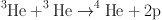 |
which completes the fusion of He. This reaction is unusual in that it actually increases the number of particles per volume, starting with two particles and producing three. The mass is the same and the reaction reduces μ locally. This is a very small effect, and it is usually swamped by the other fusion reactions that occur in a H-burning region. But here, this is the fastest reaction and it rapidly produces a μ inversion. This should initiate mixing. Further, it occurs just as the H shell approaches the discontinuity in the composition left behind by the FDU, i.e., it occurs just at the position of the LF bump, in accord with (most) observations. This mechanism has many attractive features because it is based on well-known physics, occurs in all low-mass stars, and occurs at the required position on the RGB (Charbonnel & Zahn 2007b; Eggleton, Dearborn, & Lattanzio 2008).
 |
Figure 12. Abundance profiles in a 0.8 M⊙ model with Z = 0.00015 (see also Figure 9). The left panel shows a time just after core hydrogen exhaustion and the right panel shows the situation soon after the maximum inward penetration of the convective envelope. At this time the hydrogen burning shell is at m(r) ≈ 0.31 M⊙ and the convective envelope has homogenised all abundances beyond m(r) ≈ 0.36 M⊙. The initial 3He profile has been homogenised throughout the mixed region, resulting in an increase in the surface value, which is then returned to the interstellar medium through winds, unless some extra-mixing process can destroy it first. |
Having identified a mechanism it remains to determine how to model it. Eggleton et al. (2006, 2008) preferred to try to determine a mixing speed from first principles, and try to apply that in a phenomenological way. Charbonnel & Zahn (2007b) preferred to use the existing theory of Ulrich (1972) and Kippenhahn et al. (1980). Both groups found that the mechanism had the desired features, in that it began to alter the surface abundances at the required observed magnitude, it reduced the C isotope ratio to the lower values observed, and it destroyed almost all of the 3He produced in the star, thus reconciling the predicted yields of 3He with observations (Eggleton et al. 2006; Lagarde et al. 2011, 2012), provided the free parameter C was taken to be C ≈ 1 000. Further, mixing reduced the A(Li) values as required by observation and it also showed the correct variation in behaviour with metallicity, i.e., the final 12C / 13C ratios were lower for lower metallicity (Eggleton et al. 2008; Charbonnel & Lagarde 2010).
An extensive study of thermohaline mixing within rotating stars was performed by Charbonnel & Lagarde (2010). They found that thermohaline mixing was far more efficient at mixing than meridional circulation, a result also found by Cantiello & Langer (2010). Note that the latter authors did not find that thermohaline mixing was able to reproduce the observed abundance changes on the RGB, but this is entirely due to their choice of a substantially lower value of the free parameter C (see also Wachlin, Miller Bertolami, & Althaus 2011). Cantiello & Langer (2010) also showed that thermohaline mixing can continue during core He burning as well as on the AGB, and Stancliffe et al. (2009) found that it was able to reproduce most of the observed properties of both C-normal and C-rich stars, for the ‘canonical’ value of C ≈ 1 000.
The interaction between rotation and thermohaline mixing is a subtle thing, yet both Charbonnel & Lagarde (2010) and Cantiello & Langer (2010) treated this crudely, by simply adding the separate diffusion coefficients. This is unlikely to be correct and one can easily imagine a situation where rotation, or any horizontal turbulence, could decrease the efficiency or even remove the thermohaline mixing altogether. Indeed a later study by Maeder et al. (2013) showed that simple addition of the coefficients was not correct and these authors provide a formalism for simultaneously including multiple processes. Calculations using this scheme have not yet appeared in the literature.
For a more detailed comparison of predictions with data, Angelou et al. (2011, 2012) decided to investigate the variation of [C/Fe] with absolute magnitude in GCs. The C isotopic ratio saturates quickly on the RGB, whereas [C/Fe] and [N/Fe] continue to vary along the RGB, providing information on the mixing over a wide range of luminosity. They found good agreement with the thermohaline mixing mechanism, again provided C ≈ 1 000, although they also noted that standard models failed to match the FDU found in the more metal-poor GCs, such as M92. This is not a failure of the thermohaline mixing paradigm but of the standard theory itself (as discussed earlier in Section 2.3.1).
Clearly the value of the free parameter C is crucial. On the one hand, it is gratifying that so many observational constraints are matched by a value of C ≈ 1 000. However, the value is not favoured a priori by some authors. We have seen that within the formalism of the idealised one-dimensional theory of Ulrich (1972) and Kippenhahn et al. (1980), the value of C is related to the aspect ratio α of the assumed ‘fingers’ doing the mixing, with C = 8/3π2α2. If the mixing is more ‘blob-like’ than ‘finger-like’ then α ≈ 1 and C ≈ 20 rather than 1 000. This was the case preferred by Kippenhahn et al. (1980), in fact, whereas Ulrich (1972) preferred fingers with α ≈ 5 leading to C ≈ 700, much closer to the value of 1 000 that seems to fit so many constraints. We would caution against a literal interpretation of the aspect ratio and finger-like nature of the mixing. The one-dimensional theory is very idealised and we feel it is perhaps wise to remember that the diffusion equation is a convenient, rather than accurate, description of the mixing.
Even if we assume that the mechanism identified by Eggleton et al. (2006) is the one driving extra mixing, it is unsatisfactory having an idealised, yet approximate, theory that still contains a free parameter. We need a detailed hydrodynamical understanding of the process. Studies along these lines have begun but a discussion of that would take us far afield from our main aim in this paper. We refer the reader to the following papers for details: Denissenkov, Pinsonneault, & MacGregor (2009), Denissenkov (2010), Denissenkov & Merryfield (2011), Traxler, Garaud, & Stellmach (2011), Rosenblum et al. (2011), Mirouh et al. (2012)), and Brown, Garaud, & Stellmach (2013). Let us summarise by saying that the models predict more blob-like structures, with low values of α and C values too small to match the observations. The stellar regime is difficult for simulations to model accurately and the final word is not yet written on the subject.
To summarise, thermohaline mixing occurs naturally at the appropriate magnitude on the RGB and it provides the right sort of mixing to solve many of the abundance problems seen on the RGB, as well as the 3He problem. One area where the thermohaline mechanism is open to criticism is its prediction that low-mass stars should almost completely destroy 3He and yet there are known planetary nebulae (PNe) with large amounts (i.e., consistent with the standard models) of 3He present, as pointed out by Balser, Rood, & Bania (2007, see also Guzman-Ramirez et al. 2013) immediately after the paper by Eggleton et al. (2006). Charbonnel & Zahn (2007a) suggested that perhaps an explanation could be related to magnetic fields and identified the few percent of stars that do not show decreased C isotopic ratios with the descendants of Ap stars. They showed that remnant fields of order 104 - 105 Gauss, as expected from Ap stars when they become giants, are enough to inhibit thermohaline mixing.
2.3.5. Magnetic fields and other mechanisms
Despite its many appealing features, thermohaline mixing still suffers from at least one major problem: hydrodynamical models do not support the value of C required to match the observations. This leads to the search for other mechanisms.
One obvious contender is magnetic fields (Busso et al. 2007) produced by differential rotation just below the convective envelope. This can produce a toroidal field and mixing by magnetic buoyancy has been investigated by various authors (e.g., Nordhaus et al. 2008; Denissenkov et al. 2009).
In contrast, Denissenkov & Tout (2000) suggested that a combination of meridional circulation and turbulent diffusion could produce the required mixing. These authors found that the rotation rates required were reasonable but we note that the best models of rotating stars at present do not produce enough mixing.
The behaviour of lithium is complex and deserves a special mention. The main isotope of lithium, 7Li, is destroyed by H burning at relatively low temperatures (T ≳ 2.5 × 10⁶ K or 2.5 MK) and as such is observed to be depleted during the pre-main sequence phase (see, for example, Yee & Jensen 2010; Eggenberger et al. 2012; Jeffries et al. 2013). The FDU acts to further reduce the surface lithium abundance through dilution with material that has had its lithium previously destroyed. It then appears to be further destroyed by extra mixing above the bump on the RGB. The behaviour of Li in the GC NGC 6397 was discussed earlier in Section 2.3 and is shown in Figure 9.
The situation with Li is complicated by the existence of Li-rich K-giants (Charbonnel & Balachandran 2000; Kumar, Reddy, & Lambert 2011; Monaco et al. 2011). Approximately 1% of giants show an enhancement of Li, sometimes a large enhancement to values greater than found on the main sequence (say A(Li) > 2.4). While some studies argue that these Li-rich giants are distributed all along the RGB, others find them clustered predominantly near the bump. Palacios, Charbonnel, & Forestini (2001) suggested that meridional circulation could lead to a ‘Li-flash’ that produces large amounts of Li that are only present for a short time, making the Li-rich stars themselves relatively rare. Lithium production was found in the parameterised calculations of extra mixing by Sackmann & Boothroyd (1999), for the case where the mixing (as measured by a mass flux in their case) was fast enough. Denissenkov & Herwig (2004) also found that Li could be produced through sufficiently rapid mixing. Within the approximation of diffusive mixing, they found that a value of D ≈ 109 cm2s− 1 is required to explain the usual abundance changes beyond the bump on the RGB, but a value about 100 times larger was shown to produce Li.
It seems natural that if the Li-rich stars really are created at all points along the RGB then the cause is most likely external to the star. If this requires an increase in the diffusion coefficient then something like a binary interaction or the engulfing of a planet due to the growth of the stellar envelope may be involved (Siess & Livio 1999a, 1999b; Denissenkov & Herwig 2004; Carlberg, Majewski, & Arras 2009; Carlberg et al. 2010).
Kumar et al. (2011) argue that in fact the Li-rich giants are predominantly clump stars, involved in core He burning. They argue that the Li may be produced at the tip of the giant branch at the core flash, and then given the longer evolutionary timescales for core He burning, the stars appear to be clustered around the clump (at a similar luminosity to the bump). In addition to the cases noted above that produce Li, we note here that some implementations of thermohaline mixing also produce Li at the tip of the giant branch and that there is evidence for Li-rich stars at this phase of the evolution (Alcalá et al. 2011).
We have seen that following core He exhaustion the star begins to ascend the AGB. If the mass is above about 4 M⊙ then the model will experience the SDU where the convective envelope grows into the stellar interior. In contrast to the FDU, the SDU goes deeper and mixes material exposed to complete H burning. The main changes are listed in Table 1 and include a substantial increase in the He content by up to ΔY ≈ 0.1 as well as an increase in the 14N / 15N ratio and the 23Na abundance (Figure 6).
This huge increase in He is one of the reasons why intermediate-mass AGB stars have been implicated in the origin of the multiple populations observed in Galactic GCs (D’Antona et al. 2002; Norris 2004; Piotto et al. 2005). Increases in He and changes to the composition of the light elements C, N, and O are the most likely cause of the multiple main sequence, sub-giant, and giant branches observed in all clusters that have Hubble Space Telescope photometry (e.g., for 47 Tucanae, NGC 6397, NGC 2808, M22; Milone et al. 2012a, 2012b, 2012c; Piotto et al. 2012).
Figure 6 illustrates the effect of the SDU on the abundance of intermediate-mass stars of solar metallicity. Figure 7 shows that the depth reached by the SDU is approximately the same for all the 5 and 6 M⊙ models, regardless of the initial metallicity (Boothroyd & Sackmann 1999). The effect of the SDU on other elements is small. Boothroyd et al. (1994) showed that the O isotope ratios are essentially unchanged. Small decreases in the surface abundance of fluorine may occur by at most 10% and sodium is predicted to increase by up to a factor of ≈ 2 at the surface of intermediate-mass stars that experience the SDU (e.g., Figure 8; El Eid & Champagne 1995; Forestini & Charbonnel 1997).
2.6. Variations at low metallicity
2.6.1. Curtailing first dredge-up
At metallicities of [Fe/H] ≲ -1, the evolution of post main sequence stars begins to significantly differ to that found in disk or near-solar metallicity stars. For intermediate-mass stars the necessary central temperatures for core He burning are reached while the star crosses the Hertzsprung gap. This means that the star will ignite He before evolving up the RGB and as a consequence will not experience the FDU (e.g., Boothroyd & Sackmann 1999; Marigo et al. 2001). In Figure 13 we show evolutionary tracks for models of 3 M⊙ at a metallicity of Z = 0.02 and Z = 0.0001, respectively. The lower metallicity model skips the RGB altogether. At a metallicity of Z = 0.001 or [Fe/H] ≈ −1.2 the upper mass limit that experiences the FDU is 3 M⊙, by a metallicity of Z = 0.0001 or [Fe/H] ≈ −2.3, this mass has been reduced to 2.25 M⊙, and even at that mass the maximum extent of the convective envelope only reaches a depth of ≈ 1 M⊙ from the centre (compared to a Z = 0.02 model of 2.25 M⊙ where the FDU reaches a depth of ≈ 0.35 M⊙ from the stellar centre). Because the lower metallicity model is hotter and has a larger core during the main sequence the FDU still causes a 30% drop in the surface C abundance (compared to a drop of 36% for the Z = 0.02 model). For intermediate-mass stars that do not experience a FDU, the second dredge-up event, which takes place during the early ascent of the AGB, is the first mixing episode that changes the surface composition (Boothroyd & Sackmann 1999; Chieffi et al. 2001; Marigo et al. 2001; Karakas & Lattanzio 2007; Campbell & Lattanzio 2008).
 |
Figure 13. Hertzsprung-Russell (HR) diagram showing the evolutionary tracks for 3 M⊙ models of Z = 0.02 (black solid line) and Z = 0.0001 (red dashed line). The low-metallicity model is hotter and brighter at all evolutionary stages and does not experience a RGB phase or the first dredge-up. |
Metallicity has an important consequence for stars that experience the core He flash. Evolution at lower metallicities is hotter, owing to a lower opacity. This means that the stars experience a shorter time on the RGB before reaching temperatures for core He ignition and therefore do not become as electron degenerate. This means that the maximum mass for the core He flash decreases with decreasing Z (Marigo et al. 2001). We mentioned previously that at solar metallicity the maximum mass for the core He flash is 2.1 M⊙, whereas at [Fe/H] = − 2.3 the maximum mass is 1.75 M⊙, with the 2 M⊙ model experiencing a fairly quiescent He ignition with only a moderate peak in the He luminosity (Karakas & Lattanzio 2007; Karakas 2010).
There is now a fairly extensive literature on multi-dimensional studies of the core He flash (Deupree 1984, 1986; Deupree & Wallace 1987; Deupree 1996; Dearborn et al. 2006; Mocák et al. 2009). Early results from two-dimensional hydrodynamic simulations (Deupree & Wallace 1987) suggest that the flash could be a relatively quiescent or violent hydrodynamic event, depending on the degeneracy of the stellar model. Deupree (1996) finds for low-mass solar composition models, using improved but still uncertain input physics, that the core flash is not a violent hydrodynamic event and that there is no mixing between the flash-driven H-exhausted core and the envelope at this metallicity. More recent multi-dimensional hydrodynamic simulations of the core He flash in metal-free stars find that the He-burning convection zone moves across the entropy barrier and reaches the H-rich layers (Mocák et al. 2010; Mocák, Siess, & Müller 2011).
For the present we assume that stars experiencing the core He flash do not mix any products into their envelope. This is in accord with standard models and the observations do not disagree. We do note that this is not necessarily true at lower metallicity, as we discuss in the next section.
2.6.3. Proton ingestion episodes
The low entropy barrier between the He- and H-rich layer can lead to the He flash-driven convective region penetrating the inner edge of the (now extinguished) H-burning shell. If this happens, protons will be ingested into the hot core during the core He flash. If enough protons are ingested, a concurrent secondary flash may occur that is powered by H burning and gives rise to further nucleosynthesis in the core. The subsequent dredge-up of matter enriches the stellar surface with large amounts of He, C, N, and even possibly heavy elements synthesised by the s process. There has been an extensive number of studies of the core He flash and resulting nucleosynthesis in low-mass, very metal-poor stars (e.g., D’Antona & Mazzitelli 1982; Fujimoto, Iben, & Hollowell 1990; Hollowell, Iben, & Fujimoto 1990; Schlattl et al. 2001; Picardi et al. 2004; Weiss et al. 2004; Suda, Fujimoto, & Itoh 2007; Campbell & Lattanzio 2008; Suda & Fujimoto 2010; Campbell, Lugaro, & Karakas 2010). The details of the input physics used in the calculations clearly matter, where the low-mass Z = 0 models of Siess, Livio, & Lattanzio (2002) find no mixing between the flash-driven convective region and the overlying H-rich layers. It has been known for some time that the treatment of the core He flash in one-dimensional stellar evolutionary codes is approximate at best, owing to the fact that the core He flash is a multi-dimensional phenomenon (Deupree 1996; Mocák et al. 2011). We deal more extensively with this in Section 3.8.
1 Where Z is the global mass fraction of all elements heavier than H and He, with mass fractions X and Y respectively. Back.
2 Using the standard spectroscopic notation [X/Y] = log 10(X/Y)* − log 10(X/Y)⊙. Back.
3 Using the notation A(X) = log ε(X) = log 10(NX/NH) + 12 and NX is the abundance (by number) of element X. Back.