


Stars and star clusters form when dense gas collapses through gravitational or turbulent processes. The physical state of the gas (including temperature, pressure, metallicity, and turbulence) determines which pockets of gas fragment and collapse, and so ultimately the masses of the stars formed. Since the evolution of a single star is almost entirely determined by its initial mass (although binary effects also play a role), and the distribution of mass within a bound system defines its kinematics, the evolution of a cluster of coeval stars is determined almost entirely by its stellar IMF. The evolution of galaxy composed of such clusters depends intimately on this (potentially varying) IMF in combination with its SFH.
The IMF establishes the fraction of mass sequestered in sub-solar-mass stars (down to masses as little as 0.1 M⊙) with lifetimes much greater than the age of the Universe, and the high-mass fraction (stars up to 120 M⊙ or perhaps more) that rapidly become supernovae, returning chemically enriched gas to the interstellar medium to support subsequent generations of star formation. The less numerous higher mass stars dominate the light from a star cluster or a galaxy, but the more numerous lower mass stars dominate the mass. This results in a need for different tracers to probe the high and low mass regimes of the IMF. It also means that the mass-to-light ratio is sensitive to the IMF shape.
The IMF is consequently the fundamental concept linking each of: (1) The process of star formation itself through the conversion of molecular clouds (enriched to some degree by heavy elements) into a population of stars; (2) Feedback and chemical enrichment processes arising from the radiative and mechanical energy returned to the interstellar medium through stellar winds and supernovae from existing stellar populations, that influence subsequent generations of stars and their metallicity; (3) The measurements used to convert observables, (such as broadband luminosities or spectral line measurements), to underlying physical quantities (such as the current rate of star formation and total stellar mass), in order to enable studies of star formation and galaxy evolution.
The IMF was first measured by Salpeter (1955) while working at the Australian National University, by measuring the luminosity distribution of stars in the solar neighbourhood. It was shown to be consistent with a power law over the mass range 0.4 ≲ m / M⊙ ≲ 10. Numerous measurements of the IMF over the subsequent sixty years (e.g., Miller & Scalo, 1979, Scalo, 1986, Basu & Rana, 1992, Kroupa et al., 1993) show that this power law does not extend to the lowest masses, but has a flatter slope below about half a solar mass. The original power law slope for high mass stars found by Salpeter extends up to about 120 solar masses (e.g., Scalo, 1986, Scalo, 1998, Kroupa, 2001, Chabrier, 2003a), although with some variation (but also large observational uncertainties) in the reported high-mass slope and upper mass limit, and some debate about the value for the characteristic or “turn over” mass.
While much of the observational work on the IMF in the late 20th century focused on this same method of using resolved star counts as the most robust and direct approach available, Kennicutt (1983) pioneered an approach using integrated galaxy light. Many alternatives were also explored, as summarised by Scalo (1986) and Kennicutt (1998). These include a range of approaches such as ultraviolet (UV) luminosities of galaxies (Donas & Deharveng, 1984), indirect approaches related to chemical evolution and abundance ratios (Audouze & Tinsley, 1976), and others like galaxy mass-to-light ratios that are now more routinely used to estimate IMF properties (e.g., Treu et al., 2010).
The IMF was also used as a probe of cosmology and dark matter. For example, constraints on the IMF and cosmology were inferred from the evolution of galaxy colours (Tinsley, 1972), number counts of galaxies (Guiderdoni & Rocca-Volmerange, 1990), and the form of the IMF was invoked to explore the extent to which stellar remnants (e.g., Dantona & Mazzitelli, 1986) or substellar objects (e.g., Staller & de Jong, 1981) could explain the “missing matter” in the Solar vicinity (Bahcall, 1984). The cosmological constraints associated with the IMF are no longer compelling in the age of precision cosmology (e.g., Schmidt et al., 1998, Planck Collaboration et al., 2016). Likewise, as the numbers of substellar objects have been progressively constrained by observations (e.g., Tinney, 1993, Kroupa et al., 1993) and other approaches matured in ruling out stellar-related contributions to possible baryonic dark matter (Graff & Freese, 1996a, Graff & Freese, 1996b, Alcock et al., 2000, Alcock et al., 2001), this aspect of the IMF has also become less important. With the establishment of the now standard ΛCDM model, the focus on the IMF now is primarily connected to the physics of star formation and galaxy evolution.
Part of the challenge in understanding the IMF as currently conceived is that it is a fundamentally statistical concept, and not directly observable. Elmegreen (2009) notes that when estimating the IMF for star clusters, “no cluster IMF has ever been observed throughout the whole stellar mass range.” He explains that to probe the upper mass range of the IMF needs a very massive cluster, which are rare systems, with the nearest being too far away (a few kpc) to see the low mass stars. Conversely the nearest clusters, required for measuring the low mass end of the IMF, are all low mass clusters having few high mass stars. He concludes: “Until we can observe the lowest mass stars in the highest mass clusters an IMF makes sense only for an ensemble of clusters or stars.” It is notable that the science cases for the next generation of major telescope facilities, James Webb Space Telescope (JWST), Giant Magellan Telescope (GMT), Thirty Metre Telescope (TMT), European Large Telescope (ELT), all include the goal of studying resolved star formation in such high mass Galactic star clusters. Kroupa et al. (2013) takes this concept a step further, and details why the IMF is not ever a measurable quantity, by noting that star formation occurs on Myr timescales. This means that for stellar systems younger than about 1 Myr star formation has not ceased and so the IMF is not yet assembled, while for systems older than about 0.5 Myr higher mass stars are lost through stellar evolutionary effects, while dynamical processes can also cause the loss of lower mass stars. This means that there is no single time at which the full ensemble of masses is present and measurable within a discrete spatial volume. There is hence a need to address the issue of the short but finite time of formation, together with the fact that star clusters do not form in isolation (typically) but within a complex, multiphase interstellar medium that is also influenced by, and influencing, adjacent sites of star formation.
A possible solution to this issue arises through considering how many independent samples are required, and over what spatial scale they must be probed, in order to infer the IMF robustly. By sampling a sufficiently large number of star forming regions it might be expected that each evolutionary stage is captured and the ensemble can be used to infer the underlying IMF. Kruijssen & Longmore (2014) describe a general formalism, which they apply to star formation scaling relations in galaxies, that links the timescale of different phases of a process with the number of independent samples required to capture all temporal phases and the spatial scale on which the processes are measured. They note that “[star formation] relations measured in the solar neighbourhood are fundamentally different from their galactic counterparts” and conclude that “…when a macroscopic correlation is caused by a time evolution, then it must break down on small scales because the subsequent phases are resolved.” Considering the temporal dependencies of star formation, and the range of spatial scales over which we are interested in characterising it, it may be that the formalism and concept of the IMF itself may need to be restructured (Scalo, 1998).
Despite these difficulties, a range of the early approaches toward inferring the IMF have been refined over the past decade, and are now used routinely. These include an update of the Kennicutt (1983) approach used by Hoversten & Glazebrook (2008) and Gunawardhana et al. (2011), use of the Wing-Ford band to infer dwarf-to-giant ratio (e.g., Cenarro et al., 2003, van Dokkum & Conroy, 2010, Smith et al., 2012) following the early work of Whitford (1977), use of kinematics (e.g., Cappellari et al., 2012), gravitational lensing observations (e.g., Treu et al., 2010, Smith & Lucey, 2013), chemical abundance constraints (e.g., Portinari et al., 2004a, Komiya et al., 2007, Sliwa et al., 2017) and more. The 2.3 µm CO index has also been proposed for probing the dwarf-to-giant ratio (Kroupa & Gilmore, 1994, Mieske & Kroupa, 2008). In the same period other novel approaches have been developed, such as those using cosmic census measurements to place constraints on the IMF (e.g., Baldry & Glazebrook, 2003, Hopkins & Beacom, 2006, Wilkins et al., 2008a, Wilkins et al., 2008b).
With this explosion in the range of approaches now being used to measure or infer the IMF there has been a related growth in the tension between apparently conflicting results. One example is a need for so-called “top-heavy” IMFs (a relative excess of high mass stars compared to the nominal Salpeter IMF) in regions of elevated star formation rate (e.g., Gunawardhana et al., 2011) that contrasts with the so-called “bottom-heavy” IMFs (a relative excess of low mass stars) inferred in the cores of massive elliptical galaxies (e.g., van Dokkum & Conroy, 2012). It is less clear whether such results are actually in conflict or not. The different approaches measure different things, and the spatial scales probed are different as is the epoch for the star formation activity. The current review is aimed at assessing the available wealth of different metrics and their results in a self-consistent fashion, to begin to unify our approach to understanding the IMF.
With this context in mind it is first necessary to review the terminology used in discussing the IMF and to explore conventions of nomenclature.
2.2. IMF definitions and terminology
At its most concrete the IMF can be defined as the mass distribution of stars arising from a star formation event. It has been described and inferred in this sense from observational measurements by innumerable authors over more than 60 years (e.g., Salpeter, 1955, Miller & Scalo, 1979, Kennicutt, 1983, Scalo, 1986, Kroupa, 2001, Chabrier, 2003a), who have found that the IMF in many cases follows a similar form, and established the broad properties of this distribution. In general, the IMF has a declining power-law shape for masses above about 1 M⊙, with a flatter slope at lower masses down to some minimum mass. Below the stellar/sub-stellar boundary brown dwarfs are often now included in IMF estimates (e.g., Kroupa et al., 2013), with a more positive slope below the hydrogen burning mass limit (although the shape at the lowest masses may be more complex, e.g., Drass et al., 2016). The observed mass function across the stellar/sub-stellar boundary may be a superposition of two physically distinct IMFs, inferred from the deficit in models compared to observations of brown dwarfs that form through direct gravitational collapse in molecular clouds (Thies et al., 2015). The general shape and key parameters of the IMF are illustrated in Figure 1.
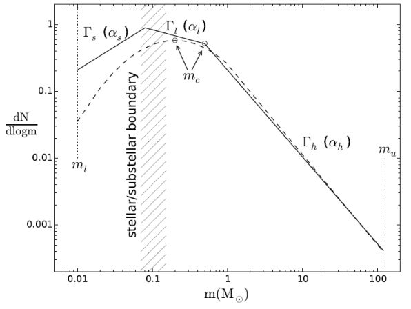 |
Figure 1. An illustration of the key aspects of the IMF as it has been parameterised, either as a piecewise series of power-law segments (e.g., Kroupa, 2001) or a log-normal at low masses with a power-law tail at high masses (e.g., Chabrier, 2003a). |
Many authors have summarised the range of functional forms used to parameterise the IMF, with the common choices being piecewise power laws (e.g., Kroupa et al., 2013, their Equations 4 and 5) or a log-normal form (e.g., Chabrier, 2003b, 2005). Alternative functional forms have been proposed with varying motivations (e.g., De Marchi et al., 2005, Parravano et al., 2011, Maschberger, 2013) that largely provide the same practical functionality as the more commonly used forms.
Key parameters are: (1) the lower mass limit, ml, typically chosen as ml = 0.08 M⊙ or ml = 0.1 M⊙ (unless substellar objects are included, in which case ml = 0.01 M⊙ is common); (2) the upper mass limit, mu, with typical values of mu = 100 M⊙, mu = 120 M⊙ or mu = 150 M⊙; (3) mc, the characteristic mass, which is the peak in the lognormal form, or the “turn over” mass where the slope of the power law representation changes (although as seen in Figure 1 this isn't necessarily an actual turn over in the relation), with mc ranging from about 0.2 M⊙ to 1 M⊙ depending on the formalism chosen, and mc = 0.5 M⊙ common in the power law representation; (4) the slope parameters for each segment of a piecewise power law relation, or the equivalent in the lognormal relation defining the width of the relation at low masses, and the power law slope at high masses. Here and throughout I use αs for the substellar power law slope, αl for the low mass slope, and αh for the high mass slope (noting mc for clarity when relevant). This choice avoids a numerical sequence in which α1 (say) is ambiguous depending on the value of ml, i.e., whether the IMF in question includes substellar masses or not. Where a single power-law spanning more than one of these segments is assumed, I use α and define the mass range explicitly.
The same functional form for the mass distribution of stars formed in a single star forming region and called “the IMF”, is also used to describe the average mass distribution of stars formed across a galaxy, a concept sometimes referred to as the “integrated galaxy IMF” or IGIMF (Kroupa & Weidner, 2003), as well as to the effective average stellar mass distribution for a population of galaxies, referred to as the “cosmic IMF” (Wilkins et al., 2008b). If the IMF is universal these quantities may be identical 2 but not otherwise. Such broad application of the term “IMF”, validated through an underlying presumption of an IMF that is “universal” until proven otherwise, may actually be hampering attempts to further understand the properties of the IMF including whether or not it varies. I return to this point below in § 2.4 and § 8.
Other issues that hamper progress arise from inconsistent conventions describing the IMF. This field suffers from a wide range of such inconsistencies, and these seem to be growing in number rather than converging as the breadth of investigations increases. In an effort to stem this flow I explicitly address these next.
2.3. Conventions and language usage
Ambiguities in the way the IMF is discussed unnecessarily complicate what is already a complex problem. Different authors adopt different conventions or approaches to the description of the IMF. Different language is used to describe the same quantity, mass ranges are omitted or assumed implicitly, and ambiguous terms are introduced. While not a fundamental problem, this definitely leads to confusion and the potential for misinterpretation, which can be easily avoided if clear conventions and unambiguous language are used. That this point has been made repeatedly by different authors (e.g., Kennicutt, 1998, Bastian et al., 2010), and still bears repeating is evidence that it deserves attention. Similar issues of convention and usage have been recognised by the cosmology community (Croton, 2013), emphasising the importance of striving for clarity.
Here I recount a number of sources of potential confusion and make recommendations for avoiding ambiguity, while acknowledging that the majority of authors do tend to be diligent. The bottom line, though, is that because of the many potential sources of confusion in this field there is an especial need for authors, referees and editors to make extra effort to ensure clarity and consistency.
Different authors have adopted a variety of nomenclature to represent the shape and power law slope(s) of the IMF, and in particular whether or not a negative sign is given in the power law definition or appears in the parameter. Opposing sign conventions may even appear within a single publication (e.g., Elmegreen, 2009, Turner, 2009). This can lead to unnecessary confusion, especially when discussing the exponent of a power law slope in a distribution that has opposite signs at the low mass and high mass ends. It is worth noting that opposing conventions for the use of the negative sign have existed almost as long as work in this field. Salpeter (1955) did not use a pronumeral descriptor for the power law slope at all, but provided the power law value explicitly in his Eq. 5, a choice followed by Kennicutt (1983). Audouze & Tinsley (1976) and Tinsley (1977) give the negative sign in the equation, a choice subsequently recommended by Kennicutt (1998), but Miller & Scalo (1979), Scalo (1986), and Kennicutt et al. (1994) use the convention that any sign is incorporated into the slope parameter.
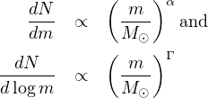
I strongly recommend that, to minimise ambiguity, all authors adopt the latter convention (following, e.g., Scalo, 1986, Kennicutt et al., 1994):
 |
(1) (2) |
where Γ = α + 1 and the original Salpeter slope is α = −2.35 or Γ = −1.35. Contrary to some recent usage (e.g., Bastian et al., 2010, Kroupa et al., 2013), the negative sign is not included in the relations adopted here, and appears in the quantities α and Γ explicitly. This convention has the advantage that the sign of the parameter and of the power law itself are the same, not opposing. It ensures that a sign change from the lowest masses to the highest masses (in a piecewise power law description, for example) is in the sense that intuition would suggest. It avoids inconsistencies or clumsy presentation when discussing the value of the power law slope as contrasted with the value of the parameter, or when inequalities are used to describe slopes flatter or steeper than some nominal parameter value. It eliminates confusion over the need to swap the sense of asymmetric errors in estimates of the parameter as opposed to the actual slope. For internal self-consistency and ease of comparison between published results, I present all IMF slopes discussed throughout using α as defined above.
The use of the phrases “Salpeter IMF,” “universal IMF,” “typical IMF,” “normal IMF,” or “standard IMF”, often interchangeably, can be confusing because of the varying assumptions made in relation to the stellar mass range and whether or not a slope change is assumed at the low mass end. Sometimes what is meant is the Salpeter power law slope over a given mass range (typically 0.1 < (m / M⊙) < 100), but also sometimes extending up to 120−150 M⊙, and often including other implicit assumptions. Common omissions that lead to ambiguity include the mass range being assumed, the existence or degree of a change in IMF slope at low masses (a “low mass turn over”), and what the characteristic mass of such a slope change may be. Clearly in order to avoid such confusion an explicit definition for such terms should be given when they are introduced, ironically also including the phrase “the Salpeter IMF” itself, since that terminology has been used to describe all the above scenarios by different authors.
The use of the phrase “universal IMF” to mean a Salpeter IMF also leads to or reinforces the unhelpful preconception of the IMF as a physically universal quantity, and this may act as a stumbling block to further investigation (see § 2.4 below). I recommend that using the phrase “universal IMF” as a descriptor of an assumed IMF in publications be avoided, and that reference to the assumed IMF be given explicitly, to minimise ambiguity and to limit the impact on preconceptions.
It is critical to include the stellar mass range over which an IMF is being probed or discussed. This is necessary to allow comparisons between different work, which may otherwise lead to spurious differences because of different assumptions about mass ranges, either over the full (assumed) range of the IMF, or over a low or high mass sub-section. Because of implicit assumptions about the relevant mass range (frequently 0.1 < m / M⊙ < 100 but not always, often defined by the choice of SPS code being employed, and commonly related to assuming a “Salpeter IMF”) it is sometimes omitted, occasionally throughout an entire publication (e.g., those focused on the ratio of stellar to dynamical mass-to-light ratios, e.g., Treu et al., 2010, Smith & Lucey, 2013, McDermid et al., 2014). Sometimes, while not mentioned explicitly, the mass range may be implied, such as through reference to the IMF chosen in a population synthesis model (e.g., Oldham & Auger, 2016), or through mention of the comparison of total mass-to-light ratios between different assumed IMFs (e.g., Smith & Lucey, 2013). The specification of the mass range of interest should be given explicitly to avoid ambiguity.
Language describing mass ranges can quickly become ambiguous if the context is omitted (or described early and not reiterated). A study of the low mass end (m ≲ 1 M⊙) of the IMF that discusses “high mass” stars or the “high mass end” of the IMF or luminosity function probably means stars above the characteristic mass, extending up to a solar mass or so. This, though, can easily be misinterpreted by a casual reader to refer to stars well above 1 M⊙ and lead to confusion regarding the truly high mass end of the IMF. Even using “high mass” to mean stars with M ≳ 1 M⊙ (e.g., Offner et al., 2014) can be misleading. Clarifying by adding a mass range explicitly avoids such ambiguities.
There is a related ambiguity that may occur when discussing stellar masses given the sometimes significant change between initial and final masses of high mass stars (m ≳ 10 M⊙) that undergo rapid mass loss through stellar evolutionary processes. This issue is less prevalent, but has the potential to be problematic when linking an observed mass function, called the “present day mass function” (PDMF), to the IMF, or in star formation simulations.
The IMF has traditionally been estimated by measuring the stellar luminosity function from which the PDMF can be calculated. For low mass stars with lifetimes longer than a Hubble time, the PDMF is equivalent to that segment of the IMF, giving the potential for conflating the IMF and the PDMF, and made especially confusing when mass ranges are omitted from the discussion. It is not uncommon to see IMF and PDMF used interchangeably in studies of the subsolar IMF. Given the direct link between the luminosity function and the PDMF, this even leads to the potential for conflating the observed luminosity function with the IMF in discussions of the two. This is reinforced by the choice of some authors to publish mass functions with mass decreasing (rather than increasing) to the right in a diagram, to maintain the explicit link to the underlying luminosity function 3.
There is ample potential for confusion when describing an IMF slope or shape if language is not chosen carefully. Any description of a power-law relationship that is expressed variously in linear or logarithmic units needs to be cautious with words like “steep/flat (or shallow)”, “increasing/decreasing slope”, “upturn/downturn”, or “turn over”. Bastian et al. (2010) notes that an IMF that is “flat” in logarithmic mass bins will still be steep if expressed in linear mass bins (Γ = α + 1). Likewise, a “turn over” apparent in logarithmic units may not be a “turn over”, merely a change in slope, if illustrated in linear units. Particularly confusing are descriptions referring to “increasing/decreasing value of power-law index”, given the explicit ambiguity around whether the negative sign is included in the definition of the index or not. Using terms such as “steeper/flatter” or “more positive/negative slope” instead may be helpful here, but still need to be worded carefully, and can be aided by showing the power law value explicitly. Carefully worded clarification around all such descriptors is necessary to avoid ambiguity, such as being explicit about the binning scheme used, referring to changes in slope rather than “turn overs”, being clear about the mass range referred to and whether any “increase/decrease” is in the higher or lower mass direction, and so on.
With extensive and growing discussion of IMF variations there has been an associated growth in the verbal and written shorthand evolving to describe such variations. Commonly seen terms include “top-heavy”, “bottom-heavy” or “bottom-light” (but rarely “top-light” for some reason), “dwarf-rich”, “Diet-Salpeter”, “heavyweight”, and even “obese” and “paunchy” (Fardal et al., 2007). This growing range of terminology is often not well defined and can lead to confusion, such as, for example, interchanging between “bottom-heavy” and “dwarf-rich”, or the explicit ambiguity between “bottom-light” and “top-heavy”. Davé (2008) makes the distinction that “top-heavy” refers to an IMF that has a high mass slope less steep than the local Salpeter value, with “bottom-light” refering to an IMF with a Salpeter high mass slope but having a deficit of low mass stars. Avoiding such terminology in favour of simply citing the relevant power-law slope, or range of slopes, for the given mass range, would eliminate potential ambiguity completely.
New quantities are sometimes labelled using pronumerals that confusingly duplicate existing conventions. One example is the introduction by Treu et al. (2010) of an “IMF mismatch” parameter, called α, to compare mass-to-light ratios (M / L = Υ) inferred through different observational approaches (gravitational lensing and dynamics as opposed to SPS). This α is not the same as that in common use to describe an IMF power law slope, although it is directly related, and is consequently an obvious source for potential ambiguity. Clearly it is impossible to avoid duplication of all variable names, but avoiding common and clearly related choices is strongly recommended. To avoid this ambiguity while retaining the connection to the originally published nomenclature, I adopt αmm = ΥLD / ΥSPS for the “IMF mismatch” parameter throughout.
There are degeneracies in the way that an IMF can be parameterised. Perhaps the best example are the very similar shapes defined by the IMFs of Kroupa (2001) and Chabrier (2003a), although with completely different parameterisations. There can be more subtle degeneracies between parameters within a given choice of parameterisation, too, such as that between αh and mu or mc (e.g., Hoversten & Glazebrook, 2008, Gunawardhana et al., 2011). When only the total mass normalisation is constrained, there is further freedom in specifying the IMF shape, as discussed by Cappellari et al. (2013). It is important for authors to acknowledge such degeneracies and to explore the degree to which any inferred IMF parameters may be influenced.
Misuse of terminology is always a potential source of ambiguity. For example, the extensive erroneous use of the terms “bimodal” and “unimodal” to refer to an IMF shape comprised of a double or single power-law respectively (e.g., Vazdekis et al., 1996, La Barbera et al., 2013, Podorvanyuk et al., 2013). The term “bimodal” implies two overlapping distributions with recognisable “modes” or peaks, such as the model proposed by Larson (1986). Composite power-law relations do not have this characteristic and should be referred to differently.
To conclude this discussion, while these concerns may appear as some combination of obvious, trivial or nit-picking, the fact that pleas for clarity in presentation have been repeatedly published by leaders in the field over a span of decades implies a real need for care in this area. Including a statement in the final paragraph of a paper’s introduction, where it has become common to include assumptions regarding the choice of cosmological parameters, choice of magnitude system, and others, that adds assumptions about ml, mu, and IMF slope(s) or form, would go a long way to mitigating ambiguities.
Another area which deserves attention, due as much to its subtle impact as to any overt ambiguity, is the concept of “universality” of the IMF, which I address next.
2.4. The confusion wrought through “universality”
There are few areas of astrophysics as emotionally charged as the argument over whether the IMF is “universal,” that is, the same unchanging distribution regardless of environment and over the entirety of cosmic history. With conflicting lines of evidence and apparently inconsistent conclusions, emotional attachments to a particular viewpoint, as opposed to evidence-based conclusions, easily develop and can strongly influence discussion in person and also in published work. Such an environment by itself makes work in this area challenging and can limit the depth or scope of investigations and interpretation, independent of any actual observational limitations.
In the absence of compelling evidence to the contrary the IMF is typically assumed to be universal. Partly this is an issue of convenience, as it makes interpreting the observations of galaxies easier and allows the direct calculation of quantities such as stellar mass and star formation rate (SFR) that can then easily be compared among galaxy populations and over cosmic history. Also, there is generally an understandable reluctance to invoke the more complex scenario of an IMF that varies if it is not warranted, and a strong aversion to what is sometimes characterised as giving the theorists and simulators yet more free parameters to play with. Given this underlying tendency to default to the “universal” assumption, there is a preferential inclination for authors to present results as being consistent with a “universal” IMF, rather than using measured uncertainties instead to place limits on the scale of any possible variations for the given mass range, epoch, spatial scale and physical conditions being probed. This approach hampers efforts to unify IMF studies because of the need to independently extract the relevant spatial scale and other physical properties, which may not be a trivial process and serves to provide further opportunity for error. It supports a tendency to acknowlege but then dismiss a host of observational challenges in inferring the IMF (such as accounting for mass segregation, metallicity effects in the mass-luminosity relation, dynamical effects, SPS limitations, SFHs and more), by drawing a conclusion that is consistent with “universality.” This attitude may also lead to a tendency to downplay or dismiss evidence inconsistent with a “universal” IMF as arising from observational systematics or model limitations. Such results may also be relegated to the status of a special case, as with the “nonstandard IMFs in specific local or extragalactic environments” noted in the abstract of the review by Bastian et al. (2010). A related issue is that the various published IMFs for Milky Way stars can easily be conflated when arguing that observations are consistent with a “universal” IMF. As noted by Bastian et al. (2010), the Miller & Scalo (1979) and Scalo (1986) IMFs are steeper at high masses than the more recently determined Kroupa (2001) or Chabrier (2003a) IMFs (for example), and observations consistent with the former are not necessarily also consistent with the latter.
The assumption of “universality” has been questioned for about as long as the IMF has been observationally measured (see discussions in Scalo, 1986, Kennicutt, 1998, Larson, 1998), and arguments for a varying IMF have been put forward since the early 1960s (e.g., Schmidt, 1963). Much of the discussion in the 1980s and 1990s touches on the need for an evolving or variable IMF to explain a variety of puzzles, including some that still remain unresolved. These include the so-called G-dwarf problem (the deficiency of metal poor stars in the Solar neighbourhood, e.g., Worthey et al., 1996), the correlation between stellar M/L (Υ*) and Mg/H abundance in ellipticals that both increase with galaxy stellar mass (e.g., Worthey et al., 1992, Larson, 1998), the iron abundance in intracluster gas (e.g., Elbaz et al., 1995, Wyse, 1997), and others well summarised in the reviews of Scalo (1986), Kennicutt (1998) and Larson (1998). Associated with these observational lines of evidence, an extensive number of different models for varying IMFs have been proposed, both to characterise their impact on different aspects of galaxy evolution, and to explore different physical mechanisms motivating the IMF variation. While still maintaining the preference for a “universal” IMF, there developed some degree of consensus by the early 2000s that an IMF that was over-represented in high mass stars (through having a low mass cutoff at several solar masses) at early times, or in high SFR events, could explain many of these different astrophysical results (e.g., Larson, 1998, Chabrier, 2003a). Subsequently, explaining the observed 850 µm galaxy source counts with semi-analytic models (Baugh et al., 2005) required invoking such a “top-heavy” IMF in starbursts, with a flatter high mass slope (α = −1 over 0.15 < m / M⊙ < 125) compared to quiescent star formation (αl = −1.4, m < 1 M⊙, and αh = −2.5, m > 1 M⊙). This IMF modification reduces the total SFR necessary to produce the observed 850 µm flux due to the increased number of high mass stars for a given SFR (see § 7). Such a requirement continues to be developed and refined (Lacey et al., 2016), although recent observations may reduce this need somewhat (see § 6).
There are many systematics involved in estimating an IMF, though, making it challenging to unambiguously conclude that the IMF is different in different regions. This is highlighted, for example, by Massey (2011), who demonstrates that within realistic uncertainties estimates of the slope of the high mass end of the IMF in the Small Magellanic Cloud (SMC), Large Magellanic Cloud (LMC) and the Milky Way are all consistent with the Salpeter value, α = −2.35. But appealing to the “universality” of the IMF based only on the similarity of observed IMFs within nearby regions of the Milky Way or even within nearby neighbouring galaxies is not justified. The range of physical conditions being probed in these systems is limited, and does not encompass the extremes seen, for example, in starburst galaxies or in the early Universe (z > 2, say). The large observational and systematic uncertainties, too, place very broad constraints that are equally consistent with the scale of some published claims for IMF variations. The range of uncertainties for the compilation of measurements shown by Massey (2011), for example, means that those results are also consistent with the variations proposed by Gunawardhana et al. (2011), with a high mass IMF slope −2.5 < αh < −1.8, seen over a range of almost 2 dex in SFR surface density, from analysing a sample of more than 40 000 galaxies. It would be enlightening to compare local IMF results as a function of some underlying physical property directly with the extragalactic results, to see whether or not the same trends hold. This is one example of the limitations on our investigations that arise from an underlying assumption of, or a tendency to prefer a conclusion for, the “universality” of the IMF.
More than simply limiting the scope of investigation or interpretion, though, the tendency to default to an assumed “universal” IMF has other insidious effects. There is an ever-present danger for investigations to be internally inconsistent if some elements (such as an SPS model or a numerical or semi-analytic simulation) make a “universal” IMF assumption, but the analysis is testing IMF variations. Any “variation” identified must be self-consistently present in the underlying models used to infer it.
In addition, because any potential variation of the IMF means that there can be a different effective IMF as a function of spatial scale, it now becomes important to discriminate between analyses that probe the scale of star clusters, larger Hii complexes or dust and molecular gas clouds, galaxies or even entire galaxy populations. It is only relevant to compare these directly if the IMF is indeed “universal,” but if not then such comparisons may easily be misleading. Any comparison must adequately account for any putative variation with the relevant physical quantity. It also means that measured PDMFs for m ≲ 0.8 M⊙ may not necessarily correspond, as typically assumed, to the IMF (Jeffries, 2012).
There are other confusions that arise through the use of the term “universal.” It is easy, for example, to conflate the concepts of a “universal” IMF and a “universal” physical process that gives rise to an IMF that itself may or may not be “universal.” There are now numerous published models demonstrating how a common underlying physical process may lead to different IMFs (e.g., Narayanan & Davé, 2012, Hopkins, 2013b), and result in IMF variations between galaxies and as a function of time. So a “universal” physical process does not necessarily imply a “universal IMF”, and care must be taken to distinguish the two.
Occam's razor is commonly invoked by scientists because there is an elegance to the simplest possible solution, leading us to prefer not to invoke additional parameters unless clearly warranted by the data. In the case of the IMF this leads to the well-established assumption that the IMF should be “universal” in the absence of compelling evidence otherwise, but I now argue that this approach has been carried too far. It is clear that the simplest explanations are not always the most accurate or correct, although they may have the benefit of ease of use (e.g., compare Newtonian and Einsteinian formulations of gravity) and at some level the definition of “simplest is itself a subjective one. There are some physical motivators for supposing that the IMF is universal, such as the turbulent power spectrum in molecular clouds apparently having a universal form, which in turn leads to a prediction for a constant high mass IMF slope (e.g., Hopkins, 2013b). Even this argument, though, leaves open whether the low mass end of the IMF may vary. Accordingly, while there may be some physical expectation for some elements of the IMF to be universal, there is also a large selection of data that question this picture. As a consequence, I suggest that it is time to turn the basic assumption around. A better assumption would be the most general scenario, rather than the simplest, that the IMF is not universal. This approach echoes the sentiment expressed by Scalo (1998), almost twenty years ago! Many of the conclusions by Scalo (1998) are still quite pertinent today, in particular his statement that “…we are in the rather uncomfortable position of concluding that either the systematic uncertainties are so large that the IMF cannot yet be estimated, or that there are real and significant variations of the IMF index at all masses above about 1 M⊙.”
In adopting the default assumption that the IMF may be variable, we should be aiming to pose research questions that can assess how and the extent to which it varies, what physical processes are responsible, and couching discussions in language that places constraints on variations rather than merely asserting that our evidence is consistent with “universality”. Broadly adopting this attitude would lead to authors presenting the relevant physical scale, mass range, metallicity, SFR, epoch, and other relevant quantities over which their results hold, making it easier to assess the degree of consistency or not between different analyses, and improving the community’s ability to make progress in this field.
To help with this endeavour it is valuable to develop an ensemble of reference observations that provide a well defined set of boundary conditions that future measurements can be tested against. It is also critical to summarise the current state of the constraints on the IMF as a function not only of mass range, but also spatial scale, epoch and as many relevant additional physical parameters as possible such as metallicity, SFR or SFR surface density, in order to extend the visual summary introduced by Scalo (1998) and referred to by Kroupa (2002) and Bastian et al. (2010) as the “alpha plot” 4. Producing such a suite of IMF diagnostics will be invaluable in order to begin the task of quantitatively establishing whether and the degree to which the IMF may vary.
2 The IGIMF approach (Kroupa & Weidner, 2003) presents one recipe describing how a “universal” IMF may lead to different IMFs for galaxies and galaxy populations, through some star clusters being insufficiently populated at the high mass end. Back.
3 This is a direct consequence of presenting luminosity functions as a function of magnitude, rather than luminosity, as fainter magnitudes are numerically larger. This tradition arose from the original choice by Hipparchus over 2000 years ago to label the brightest stars as those of the first magnitude and counting up for fainter stars. Using modern conventions and physical units where possible should now be preferred. Back.
4 Note that each of these papers uses a different convention to describe the IMF slope, and Bastian et al. (2010) retain the terminology of Kroupa (2002) despite showing Γ rather than α! Back.