


Rather than giving extensive reviews of the many approaches that have been used in inferring IMF measurements, the intent here and in the following sections is to summarise the main outcomes from the different approaches, identify a selection of highlights, and to extract the parameter range over which the measurements are valid, in order to begin the task of unifying our understanding. In reviewing these works I draw primarily on the piecewise power-law parameterisation, using the ml, mc, mu, αl, αh notation described above. This is partly for convenience, as many of the published results use equivalent notation, but also a natural choice because analyses are often restricted to a mass range where only a single part of the piecewise power law is being constrained. Also, given the degeneracies in the way the IMF may be parameterised, it is not necessarily clear that differing measurements for a parameter (a single slope, for example) are inconsistent, unless the full parameter set is defined and can be compared between two cases.
The physical processes through which stars and star clusters form and chemically enrich their surroundings, discussed in detail by Zinnecker & Yorke (2007), Portegies Zwart et al. (2010), Tan et al. (2014), Krumholz (2014), and Karakas & Lattanzio (2014), are beyond the scope of the current review, which is aimed instead at exploring the degree to which different observational probes of the IMF are measuring the same thing. While acknowledging the fundamental underlying importance of the physics driving star formation, and relying on the results above as needed, I focus in this and the following four sections below on how we measure and use the IMF in different contexts to understand star formation and galaxy evolution.
3.1. Resolved star counts and luminosity functions
Measuring the IMF directly, even within the Milky Way and nearby galaxies where individual stars can be resolved, is challenging for several reasons, including: (1) stellar luminosities need to be converted to stellar masses, requiring information about their ages and metallicities, with more uncertainty at the low-mass end (e.g., Kroupa et al., 1993); (2) account needs to be taken of the “missing” stars, those high-mass stars that have already evolved off the main sequence, using a relation between the stellar mass and main-sequence lifetime (e.g., Reid et al., 2002, Elmegreen & Scalo, 2006); (3) assumptions need to be made for the fraction of stars that are unresolved binary systems (e.g., Bochanski et al., 2010, Luhman, 2012, De Marco & Izzard, 2017), with the intrinsic IMF slope being steeper (proportionally fewer higher mass stars) than nominally inferred if this fraction is underestimated (Scalo, 1986, Sagar & Richtler, 1991), although Weidner et al. (2009) argue that this effect is minor for high mass stars, but significant at the low mass end; (4) the degree to which mass segregation (the effect of high mass stars in a gravitationally bound system moving toward the centre of a cluster over time) affects the results in stellar clusters or associations (Zinnecker & Yorke, 2007, Tan et al., 2014, De Marchi et al., 2010). The reviews by Bastian et al. (2010), Jeffries (2012), Luhman (2012) and Offner et al. (2014) provide a more detailed discussion of these and related limitations.
Only a relatively small number of stellar systems are accessible to measure directly in this fashion, either within the Milky Way or in nearby galaxies, with many fewer being the very young systems where high-mass stars are able to be probed directly. In consequence, much of the work on the IMF in the Milky Way to date has focused on the low mass end (e.g., Jeffries, 2012, Luhman, 2012). The small number of systems available also gives rise to issues of stochasticity and sampling, which can limit the accuracy when attempting to infer the IMF for individual star clusters, associations, or dispersed field populations (Elmegreen, 1999, Kruijssen & Longmore, 2014). Apparent variations between inferred IMFs for different systems may at some level just be a consequence of these observational limitations, although De Marchi et al. (2010) argue that all star clusters in the Milky Way, young and old, are consistent with having a common underlying mass function when dynamical effects are accounted for. The IGIMF approach (Kroupa & Weidner, 2003, Kroupa et al., 2013) presents an alternative explanation, where the variations for star clusters are real and depend on, for example, a relationship between the cluster mass and the highest mass star in the cluster.
Broadly, the IMF shape for field stars in the Milky Way demonstrates a slope somewhat steeper than Salpeter (αh ≈ −2.7) at high mass (m ≳ 0.7 M⊙), with a flatter slope (αl ≈ −0.5 to αl ≈ −1) at lower masses, as summarised by Bastian et al. (2010) and Offner et al. (2014). There are many studies of the local low mass (m ≲ 1 M⊙) IMF, as reviewed by Chabrier (2003a) and Jeffries (2012) for example, but there are few Galactic studies of the field star IMF in the mass range 1 < m / M⊙ < 10. These use assumptions about the Milky Way SFH to infer an IMF with αh = −2.65 ± 0.2, as described, for example, by Bastian et al. (2010).
A limitation arises from the need to assume a recent SFH in estimating an IMF. Elmegreen & Scalo (2006) demonstrate how an assumption of a constant or slowly varying SFH can distort the inferred IMFs from observed PDMFs, if the true underlying SFH is more stochastic. In particular, an SFH decreasing with time can be misinterpreted as a steeper IMF if a constant SFH has been assumed. Elmegreen & Scalo (2006) show that this explanation can account for apparently steep IMF slopes (αh ≈ −5 ± 0.5 for 25 < m / M⊙ < 120) found for OB associations in the LMC and SMC (Massey et al., 1995, Massey, 2002). This demonstrates the need for realistic SFHs to be adopted, and for SFH uncertainties to be incorporated into uncertainties on the inferred IMF.
There are challenges in constraining the higher mass IMF (m > 1 M⊙) for the field star population due to the short lifetimes of the highest mass stars. These are best studied in OB associations and massive young clusters (e.g., Bastian et al., 2010). At m ≳ 3−10 M⊙ Offner et al. (2014) summarise recent results that suggest such star clusters and associations in the Milky Way have slopes that scatter around the Salpeter value, αh = −2.35. Mass segregation, the most massive stars tending to be found in a cluster's central regions, is often invoked as the origin of much of the scatter. Haghi et al. (2015) use simulations to argue that the lack of low mass stars observed in some globular clusters may arise through mass segregation at birth combined with the process of gas expulsion (see also Zonoozi et al., 2017, for example). If mass segregation is primordial, i.e., that the stars form in these locations, then the IMF must trivially be a variable property, although such segregation is perhaps most easily attributable to dynamical effects (Zinnecker & Yorke, 2007, Tan et al., 2014). The existence of mass segregation leads to a necessity for observations to sample sufficiently large cluster radii in estimating the IMF, in order not to be biased by the prevalence of high mass centrally located stars.
It can be seen already from this brief and incomplete summary that the broad range of observational challenges in estimating the IMF for stars in various regions within the Milky Way reinforce a tendency to invoke a “universal” IMF. There is an understandable preference to conclude that the observations are not inconsistent with a “universal” IMF, given the subtleties involved in accounting for the broad range of systematics and observational limitations.
In their review of the formation of young massive clusters, Portegies Zwart et al. (2010) conclude by noting that “globular clusters are simply old massive clusters, the logical descendants of young massive clusters in the early Universe,” a view supported by Kruijssen (2015). Zaritsky et al. (2012), Zaritsky et al. (2013), Zaritsky et al. (2014b) use the stellar mass-to-light ratios in Milky Way and Local Group stellar and globular clusters to infer, in contrast to the results above, two distinct stellar IMFs in such systems, which they describe as a “bimodal” IMF (Figure 2).
This result was initially established by measuring the stellar mass-to-light ratio in the V-band, Υ*, based on observed velocity dispersions of four key clusters (Zaritsky et al., 2012), ultimately extended to a sample of 29 clusters among 4 different host galaxies (Zaritsky et al., 2014b). The quantity Υ*,10 was introduced, being the stellar mass-to-light ratio that a cluster would have at the age of 10 Gyr, based on simple evolutionary models, in order to more accurately compare between clusters of different ages. After exploring the impact of stellar binarity on the measured velocity dispersions (Zaritsky et al., 2012), and the effects of internal dynamical evolution and relaxation driven mass loss (Zaritsky et al., 2013), they conclude that such effects are not enough to account for the observed differences in mass-to-light ratio. The resulting conclusion is that the bimodality seen in Υ*,10 is evidence for two distinct IMFs, with young stellar clusters (log(t / yr) ≲ 9.5) favouring IMFs similar to Salpeter (α = −2.35) over the full mass range (0.1 < m / M⊙ < 120 Zaritsky et al., 2012), with older clusters favouring IMFs similar to that of Kroupa et al. (1993), with proportionally fewer low mass stars, and a steeper high mass slope (αh = −2.7). They are careful to note, though, that neither of these IMFs is a unique solution, given that the constraint is on total mass arising from the measured mass-to-light ratios.
There are conflicting results regarding the mass function of globular clusters in the low mass range (m < 1 M⊙). Using mass-to-light ratios of 200 globular clusters in M31, Strader et al. (2011) find a deficit of low mass stars compared to a Salpeter slope, with −1.3 < αl < −0.8 for m < 1 M⊙ (although mass underestimates may change this conclusion, see Shanahan & Gieles, 2015). Zonoozi et al. (2016) argue that an excess of high mass stars as a function of metallicity can account for the lower than expected mass-to-light ratios of metal-rich globular clusters in M31. van Dokkum & Conroy (2011) use stellar absorption features (see § 5.3) measured for four globular clusters in M31 to infer an IMF consistent with that of Kroupa (2001), with no low mass excess. In contrast, Goudfrooij & Kruijssen (2014) show that some globular cluster systems (at least the metal-rich population) in elliptical galaxies have a low mass excess, requiring −3.0 < αl < −2.3 over 0.3 < m / M⊙ < 0.8. Zaritsky et al. (2014b) go on to show that the high and low mass-to-light ratios for their stellar clusters are well matched to those of early and late type galaxies, respectively (Figure 2), and potentially also consistent with the variations in IMF proposed for such systems (e.g., Gunawardhana et al., 2011, van Dokkum & Conroy, 2012). This suggests an observational approach that can be used for directly linking and comparing studies of stellar and galactic systems.
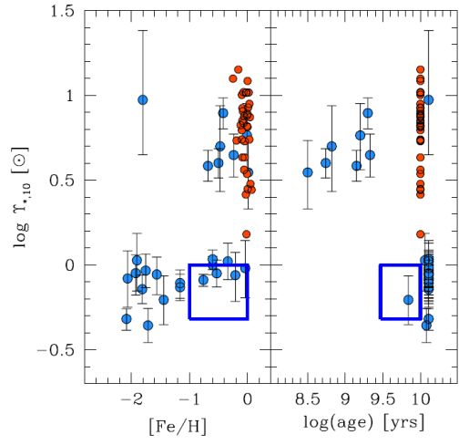 |
Figure 2. The stellar mass-to-light ratio at 10 Gyr, Υ*,10, as a function of metallicity and age, showing two distinct populations. Clusters (blue data points) with younger ages, or higher metallicities, tend to show higher mass-to-light ratios, indicative of an IMF similar to Salpeter (α = −2.35) over the full mass range. Older, more metal-poor, clusters have mass-to-light ratios consistent with an IMF having proportionally fewer low mass stars, such as that of Kroupa et al. (1993). The red data points represent the mass-to-light ratios for early type galaxies, while the blue box indicates the range of Υ*,10 for disk galaxies. See Zaritsky et al. (2014b) for details. (Figure 9 of “Evidence for two distinct stellar initial mass functions: Probing for clues to the dichotomy,” Zaritsky et al. (2014b), © AAS. Reproduced with permission.) |
Accounting for dynamical evolution is important in understanding how the observed mass function of a star cluster changes with time, and may be related to its IMF. Some simulations demonstrate that the impact of tidal fields on star clusters, or that gas expulsion from initially mass segregated globular clusters, ejects predominantly low mass stars (e.g., Baumgardt & Makino, 2003, Haghi et al., 2015). Others demonstrate the mechanisms by which star clusters can eject high mass stars (e.g., Oh & Kroupa, 2016, Banerjee & Kroupa, 2012). It is clear that there are many subtleties and details that need to be considered carefully in inferring an IMF from complex dynamically and astrophysically evolving systems.
The challenges in measuring star counts and accounting for mass segregation in star clusters when investigating the high mass end of the IMF can be sidestepped through measuring the hydrogen ionising photon rate (Calzetti et al., 2010, Andrews et al., 2013, Andrews et al., 2014). Andrews et al. (2014) demonstrate the presence of high mass stars in young (t < 8 Myr) low mass clusters (down to cluster masses of Mcl ≈ 500 M⊙) in M83. They conclude that star clusters are populated stochastically, or randomly, in stellar mass, allowing the existence of high mass stars (up to 120 M⊙) even in the lowest mass clusters (Mcl ≈ 500 M⊙), in direct contrast with the mu - Mcl relation of Weidner et al. (2010) (but see also Weidner et al., 2014). They conclude that the population of M83 star clusters they observe have a total Hα luminosity to cluster mass ratio consistent with that expected from a Kroupa (2001) IMF with 0.08 < m / M⊙ < 120.
Also exploring star clusters in a nearby galaxy, Weisz et al. (2015) have undertaken a large systematic study of the colour-magnitude diagrams for 85 young, intermediate mass stellar clusters in M31. Using a framework to infer the distribution of mass function slopes given a set of noisy measurements (Hogg et al., 2010, Foreman-Mackey et al., 2014), they find that the high mass slope of the IMF is best described by αh = −2.45−0.03+0.06, somewhat steeper than the high mass slope of Kroupa (2001) (αh = −2.3) inferred by Andrews et al. (2014). This is similar to the result of Veltchev et al. (2004) who found αh = −2.59 ± 0.09 (for m ≳ 7 M⊙) using colour-magnitude diagrams for 50 OB associations in the south-western region of M31.
The conclusions of Andrews et al. (2014) and Weisz et al. (2015) reveal part of the challenge in discussing and understanding the IMF. Both Andrews et al. (2014) and Weisz et al. (2015) present their results as being consistent with a “universal” IMF. The claim is that the IMF for the population of clusters as a whole produces an IMF consistent with that measured for the Milky Way, although the individual clusters demonstrate observed “variations”. Any of the individual low mass star clusters of Andrews et al. (2014), for example, that contain a very high mass star will necessarily demonstrate an IMF skewed to the high mass end, and be different to the IMF of other clusters in the M83 ensemble, even though their ensemble IMF is consistent with that of Kroupa (2001). Equally, the M31 cluster IMF slopes found by Weisz et al. (2015) show significant scatter individually (see their Figure 4), while the ensemble is well described by IMFs having high mass slopes drawn from a normal distribution with a very narrow intrinsic dispersion.
What the results of Andrews et al. (2014) demonstrate, but which is not made explicit, is that stochastic or random sampling of the IMF for a given cluster leads directy to variations in the IMF between clusters. The importance of stochasticity in the IMF is also highlighted by Barker et al. (2008). The ambiguity here is deeply buried in the difference between a “universal” process of star formation compared to a “universal” mass distribution produced from any given star formation event, a complication that has led to an entire industry exploring how the IMF is populated (see, e.g., discussion in Kroupa et al., 2013). The conclusions of Andrews et al. (2014) and Weisz et al. (2015) are in support of the former (a “universal” process), but not the latter. Given these consistent conclusions, the small but measurable difference in αh between M31 (Weisz et al., 2015) and M83 (Andrews et al., 2014) is worth noting. Both cases here also highlight the difference between an IMF inferred for any individual star cluster, and that for a galaxy taken as a whole, a distinction that will be a recurring theme in this review.
While Weisz et al. (2015) also use their technique to show αh = −2.15 ± 0.1 for the Milky Way and αh = −2.3 ± 0.1 for the LMC, they argue that to be robust these values would need to be calculated using the same homogeneous and principled approach as they applied to M31. They go on to recommend that their steeper αh = −2.45−0.03+0.06 slope for m > 1 M⊙ be used in the “universal” IMF shape. When calculating SFRs this IMF slope leads to values 30-50% higher than assuming the Kroupa (2001) IMF. I return to this point in § 6 below.
Other observations of starburst clusters and super star clusters provide conflicting evidence for the shape of the IMF. Such systems, containing numerous and unresolved stellar components, have been investigated using a range of techniques, including spectroscopic observations, in some cases analysed using SPS models, mass-to-light ratios and dynamics. A deficit of low mass stars has been identified in the super star cluster M82F within the galaxy M82 (Smith & Gallagher, 2001, McCrady et al., 2005, Bastian et al., 2007). The impact of a deficit of low mass stars on the dynamical evolution of such clusters appears relatively mild (Kouwenhoven et al., 2014). The Milky Way’s nuclear star cluster was analysed by Lu et al. (2013), who find an IMF slope of αh = −1.7 (for 1 < m / M⊙ < 150) and an age of around 3.3 Myr. There is evidence for a Salpeter IMF (α = −2.35 for the full mass range 0.1 < m / M⊙ < 100) in a massive young cluster in the Antennae (Greissl et al., 2010), which would imply an excess of low mass stars relative to a Kroupa (2001) or Chabrier (2003a) IMF, but other dynamical mass estimates suggest “standard Kroupa IMFs” (although without detailing which 5) in star clusters in the Antennae and NGC 1487 (Mengel et al., 2008). Banerjee & Kroupa (2012) use simulations to argue that the true IMF of R136 must have had an excess of high mass stars, given that their dynamical ejection is efficient, and that the observed mass function is consistent with that of Kroupa (2001). The early suggestions of a high value for ml in starburst nuclei (e.g., Rieke et al., 1980) have not been supported by more recent work, with Rigby & Rieke (2004) finding evidence using mid-infrared Ne line ratios for either mc ≈ 40 M⊙ (or equivalently a strong steepening in the high mass IMF slope above this value), or that high mass stars in starbursts are embedded within ultra-compact Hii regions, preventing the nebular lines from forming and escaping, the solution they favour (see also summaries by Elmegreen, 2005, Elmegreen, 2007). Recent results analysing the 30 Doradus star forming region in the LMC (Schneider et al., 2018) show strong evidence for an IMF well populated up to mu ≈ 200 M⊙, and with αh = −1.90−0.37+0.26 for 15 < m / M⊙ < 200. Taken together, such results appear to provide evidence for a relative excess of high mass stars in some, but not all, starburst clusters.
3.3. Chemical abundance measurements
Another common stellar technique used in inferring an IMF relies on the chemical abundances of stars. Since different elements are produced by stars of different mass, the present day elemental abundances can be used to infer an indirect measure of the IMF. The summary by Wyse (1998) provides an excellent overview of this approach and its issues and limitations. Broadly, oxygen and the α-elements are produced predominantly in core-collapse (Type II) supernovae, while iron is produced in both core-collapse and thermonuclear (Type Ia) supernovae. The ratio of [O/Fe] can then be used to probe the high mass star IMF, with a “plateau” in this ratio arising from stars pre-enriched only by type II SNe, the quantitative value of which would change with a change in the high mass IMF slope. A limitation is that the value of this Type II plateau depends on the theoretical yields assumed for different elements as a function of supernova progenitor mass. Wyse & Gilmore (1992) note that varying the IMF slope from αh = −2.1 to αh = −3.3 (for m > 1 M⊙) results in [O/Fe] changing by ≈ 0.4 dex, although the difference for the smaller range of −2.5 < αh < −2.1 is only Δ[O/Fe] ≈ 0.1 − 0.15 dex depending on the elemental yields assumed (their Tables 1 and 2). Wyse (1998) argues that for the Milky Way stellar halo, thick disk and bulge populations, the measured abundances are consistent with a Salpeter high mass IMF slope. A compilation of abundances was used by Nicholls et al. (2017) in introducing a new approach to scaling abundances with total metallicity, reinforcing the detection of the Type II plateau for the Milky Way, LMC and the Sculptor Dwarf (shown using [Mg/Fe], their Figure 9).
Combining abundance constraints with mass-to-light ratio constraints, Tsujimoto et al. (1997) find −2.6 < αh < −2.3 for m > 1 M⊙ for stars presently in the solar neighbourhood. They also argue for mu = 50 ± 10 M⊙, although this mu is not necessarily the highest mass of stars formed, but instead is the highest mass of stars that return chemically enriched material to the interstellar medium. In their analysis stars may exist above this mass, but those that do must end as black holes without ejecting processed material into the interstellar medium. This result has been called into question by Gibson (1998), though, who demonstrate that using different chemical yield models relaxes this outcome to a much less stringent constraint of mu ≈ 30−200 M⊙.
The chemical abundances of stars in some dwarf spheroidal (dSph) satellites of the Milky Way show measurable differences from Milky Way stars. Early work suggested that any abundance differences were still consistent with an IMF having a Salpeter high mass slope (e.g., Tolstoy et al., 2003, Venn et al., 2004). A high mass truncation of the IMF was discussed as a possible scenario to explain the differences but a solution arising from the contributions of metal-poor AGB stars was favoured. More recently, Tsujimoto (2011) argue that the deficiency of α-elements combined with an enhancement in s-process elements (Ba) found in dSph galaxies provides evidence of a lack of high mass stars (m ≳ 25 M⊙) in these systems, a result in keeping with the idea of a lower value for mu in lower SFR environments (Weidner & Kroupa, 2005). This result is supported by a different type of constraint, explored by Portinari et al. (2004a), who find that IMFs typical of the Milky Way (Kennicutt, 1983, Larson, 1998, Chabrier, 2001) can explain the mass-to-light ratios seen in Sbc/Sc galaxies but then overestimate the metallicities. They argue that unless the observed metallicity is underestimated (due to expulsion into the intergalactic medium or through being locked up in dust grains) the IMF needs to be truncated at high masses. This result was extended by Portinari et al. (2004b), showing that a “standard solar neighbourhood IMF” (Kroupa, 1998) cannot provide sufficient heavy elements to account for the observed metallicity of galaxies in clusters. None of these analyses account for galactic winds, which, if included, may help explain the observed chemical signatures without the need for the lower value of mu, although Portinari et al. (2004b) note that this would require “substantial loss of metals from the solar neighbourhood and from disk galaxies in general.”
At the other extreme, a recent analysis of starburst galaxies by Romano et al. (2017), using updated chemical models to track CNO isotopes and accounting for stellar rotation, finds a need for an excess of high mass stars (αh = −1.95, for m > 0.5 M⊙) to reproduce observed isotope abundances. This result is consistent with the conclusions of Sliwa et al. (2017) who find a need for an excess of high mass stars to explain the CO isotopic abundances in the starburst galaxy IRAS 13120-5453.
A related approach links the cosmic microwave background (CMB) to a directly observable stellar chemical signature, the carbon-enhanced metal-poor (CEMP) stars (Tumlinson, 2007), probing stars in the mass range 1 < m / M⊙ < 8. The CMB defines a temperature minimum that may translate to a characteristic fragmentation scale for star-forming gas (Larson, 2005). The time dependence of the CMB can hence have an impact on the fraction of carbon-enhanced metal-poor stars as a function of metallicity, and Tumlinson (2007) find that mc should increase toward higher redshift. This result is supported by analyses of observed CEMP stars (Komiya et al., 2007) explained as arising from binary systems, and as modelled by binary population synthesis (Suda et al., 2013). Tumlinson (2007) go on to point out that such an evolution of the IMF would lead to two clear systematic errors if it is not accounted for. Early time SFHs for local galaxies derived from colour-magnitude diagrams assuming a non-evolving IMF would be systematically underestimated, and SFRs from high-z luminosity tracers, such as UV, would be systematically overestimated. I return to these points in § 6 below.
While constraints from stellar chemistry in this fashion may turn out to be quite powerful probes of the IMF, in particular its properties at high redshift, it would be valuable to explore how limitations or systematics in our understanding of stellar yields and binary star evolution may influence or limit such measurements. One of the important potential advantages of stellar chemistry, and in particular the most metal-poor stars, is their potential for probing the first generation of stars, called “Population III” stars (Frebel, 2010), through the preserved signatures of their supernova chemical yields in subsequent generations of stars. I briefly discuss this next.
Simulations and physical arguments have demonstrated for many years that Population III stars are likely to be dominated by high mass objects (e.g., Abel et al., 2002, Bromm et al., 2002), with typical masses m > 100 M⊙ and few or no low mass stars (see review by Bromm & Larson, 2004, and references therein). Further work has explored the impact of such Population III star properties for the earliest generations of galaxies (Bromm & Yoshida, 2011). The physical processes involved are also summarised well, in the broader context of structure formation and evolution, by Loeb (2006). More recently, some simulations now appear to extend the lower mass limit for Population III stars to lower values (e.g., Hirano et al., 2014, Susa et al., 2014). Clearly the IMF for such a population would be radically different to that in the local Universe and in that sense there is trivially an evolution in the IMF. This does not address the question that is usually meant regarding the “universality” of the IMF, though, which instead is focused on whether the IMF may be different between coeval galaxies, or between different star forming regions within a galaxy. With that in mind, it is instructive to briefly touch on some of the results associated with the current measurements probing Population III stars.
Observational probes of the first stars are summarised in the review by Bromm & Larson (2004), who highlight their reionisation signature, chemical enrichment of subsequent stellar generations (“stellar archaeology”), and gamma-ray bursts as opportunities then developing. This builds on a significant body of earlier work to explore and explain the lack of low metallicity stars in the Milky Way and its halo (e.g., Bond, 1981, Jones, 1985, Cayrel, 1986) and other novel probes of Population III stars (e.g., Tarbet & Rowan-Robinson, 1982). Subsequently, gamma-ray bursts have been used to constrain the high-z SFH (Yüksel et al., 2008, Kistler et al., 2009, Kistler et al., 2013), finding a higher value of the SFR density for z > 5 than commonly inferred from deep imaging data (see summary in Madau & Dickinson, 2014), with implications for reionisation (Wyithe et al., 2010), although with no direct constraints yet on the Population III IMF. Ma et al. (2015) show that none of the gamma-ray bursts detected at 5 ≲ z ≲ 6 show abundance ratios consistent with an environment dominated by Population III stars. Opportunities for probing the first stars through stellar archaeology are summarised by Frebel (2010) and in an extensive review by Karlsson et al. (2013). Strong abundance ratio signatures are expected, with Heger & Woosley (2010), for example, demonstrating that increasing ml from 10−40 M⊙ strongly suppresses the production of elements heavier than aluminium.
Other observations are now starting to constrain the possible IMF shapes for this earliest generation of stars. Sobral et al. (2015) argue for a “flat or top-heavy IMF” (lacking stars below 10 M⊙) for Population III stars in a high-redshift (z = 6.6) Lyα system, although Bowler et al. (2017) dispute this conclusion based on deeper infrared observations. They argue for a low mass narrow-line active galactic nucleus or low metallicity starburst to explain the observed infrared colours. Fraser et al. (2017) uses abundances in extremely metal poor stars to infer a Salpeter IMF slope, αh = −2.35−0.29+0.24, with a maximum supernova progenitor mass of m = 87−33+13 M⊙ and a value of ml below the minimum mass for Population III supernovae (ml ≲ 9 M⊙). Hartwig et al. (2015) demonstrate a technique for constraining the lower mass limit of Population III stars, finding that they can exclude stars with m < 0.65 M⊙ at 95% confidence.
Future observations hold great promise for constraining the high-z IMF. Using simulations, de Souza et al. (2014) show that a few hundred supernovae detections with the JWST could be sufficient to discriminate between a “Salpeter and flat mass distribution for high-redshift stars”. Jeřábková et al. (2017) demonstrate the redshift dependent photometric properties of globular clusters and ultra-compact dwarf galaxies to provide observable IMF diagnostics for anticipated JWST observations.
With this review focused primarily on the consistency of approaches to observational constraints of the IMF I do not discuss Population III stars further. It is clear that this area will see rapid growth of a variety of observational constraints in the near future, and I hope that the framework presented here will be applied to these approaches to aid in understanding this earliest generation of stars.
With the broad range of approaches, techniques and results described above it is worth briefly summarising. Star clusters sample physical scales on the order of a few pc and a broad range of ages and SFRs, although most of those observed are high SFR surface density objects. The field star population in principle probes the full galaxy-wide scale (tens of kpc), and is sensitive to the galaxy-wide SFH.
Although the large uncertainties and systematics involved in these measurements understandably lead to a conclusion that the IMFs are all similar and broadly consistent with (for example), the IMFs of Kroupa (2001) or Chabrier (2003a), it is tantalising to note that the field star and stellar association population have high mass (m > 1 M⊙) slopes on average somewhat steeper (αh ≈ −2.5) than the cluster stars (αh ≈ −2.2, see Figure 2 in Bastian et al., 2010). The populations of globular clusters and extragalactic star clusters, in contrast, show evidence for some differences between IMFs. Probing spatial scales on the order of pc, a range of IMFs are inferred, with some globular clusters consistent with the IMF of Kroupa et al. (1993) and its steeper high mass slope (αh = −2.7), and others consistent with a Salpeter slope over the full mass range extending to the lowest masses. It is worth noting the link between the mass-to-light ratio approaches for globular clusters and galaxy systems as a technique that may lend itself to being applied self-consistently across a broad range of different physical scales and conditions.
Extragalactic star clusters demonstrate IMFs consistent with Kroupa (2001) in M83 (αh = −2.3), or with high mass slopes somewhat steeper (αh = −2.45) in M31. While this difference is small, the level of precision of these results begins to suggest that it is not negligible. At least some starburst and super star clusters tend to show evidence for an excess of high mass stars, either through an increase in mc or a flatter αh compared to the IMF of Kroupa (2001). Approaches using abundance measurements reinforce the slightly steeper high mass slope seen in field stars, and further suggest the possibility that the high mass limit mu may need to be somewhat lower than the typical Milky Way value in nearby dSph galaxies.
Taken as a whole, while the range of uncertainties and systematics makes it easy to assert that there is no strong evidence measured for IMF variations, adopting the converse approach of placing constraints on the scale of possible variations opens a different line of argument. Referring below to the Kroupa (2001) or Chabrier (2003a) IMF as the “typical” IMF for the Milky Way, it can be said that:
It is worth recalling here that there may be degeneracies between mu and αh, and that the measured constraints may be able to be reproduced by different parameter combinations. It remains the case, though, that there does appear to be some difference between the form of the IMF in high and low SFR regions. These lines of evidence suggest that the IMF is not “universal”, but that there are differences in different regions, although the details are only qualitatively constrained.
5