


The other word that is much heard when discussing the CMB is “anomalies”. What is meant here is a feature (at a low level of significance) that appears to be unexpected in the SMC, pointing to perhaps some kind of non-Gaussianity or breaking of statistical isotropy. There are several examples that have been suggested over the years, with different researchers claiming importance for one or other. Table V gives a partial list. It seems extremely hard to believe that all of these are pointing to deficiencies in the conventional picture. One should be skeptical of each of them, particularly because of the issue of a posteriori statistics. This issue is one that causes enough debate among cosmologists, that I'm going to discuss it in some detail.
| Low quadrupole and other low-ℓ modes |
| Deficit in power at ℓ ≃ 20–30 |
| Low variance |
| Lack of correlation at large angular scales |
| The Cold Spot |
| Other features on the CMB sky |
| Hemispheric asymmetry |
| Dipole modulation |
| Alignment of low-order multipoles |
| Odd-even multipole asymmetry |
| Other features in the power spectrum |
The problem is that all of these “anomalies” had their statistical significance assessed after they were discovered. Hence, in order to fairly determine how unlikely they are, it is necessary to consider other anomalies that may have been discovered instead. Statisticians call this the “multiplicity of tests” issue, which I think is the most helpful way to think about it.
Let's take the so-called CMB Cold Spot as an example (as shown in the left-hand panel of Fig. 6). The probability of finding a cold region of exactly this size and shape in exactly this particular direction is obviously vanishingly small. No one would consider such a calculation to be useful, and at the very least would appreciate that the spot could have been found in any direction – hence to assess the significance one could look in simulated skies for similarly extreme cold spots that occur anywhere. The probability determined in this way then becomes of order 0.1 %. However, a specific scale was chosen for the spot, or to be more explicit, a filter of a particular shape and scale was chosen. It turns out that the Cold Spot isn't very extreme if a purely Gaussian filter is used, but is pulled out at higher amplitude by a “compensated” filter (e.g. what is often called a “Mexican hat”) with a scale of about 5∘. This means that one should marginalise over the scale (within some reasonable bounds) and over a set of potential filter shapes (that one might have chosen) as well. On top of all this it's obviously clear that one needs to consider hot spots as well as cold spots (this may seem so self-evident that it doesn't need to be stated, but in fact several papers have only assessed the significance of cold spots). And the situation is more complicated than that, since if there had been a fairly conspicuous pair of neighbouring spots, or a hot spot diametrically opposite a cold spot, or even a triangle of spots, then one might equally well have been writing papers about the anomalous feature that was discovered.
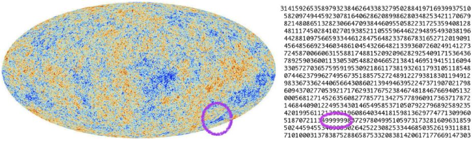 |
Figure 6. Left: map of the CMB sky from Planck, with the position of the so-called “Cold Spot” indicated. Right: the first 900 digits of π, showing the “hot spot” of six 9s (also known as the Feynman point). |
The point is that in each Hubble patch (with the CMB sky being an independent realisation of the underlying power spectrum), there will be features on the sky or in the power spectrum, that appear anomalous. One has to consider the set of potential anomalies in each patch in order to assess whether a feature is extreme enough to get excited about. In practice 2–3 σ anomalies go away when you marginalise over these possibilities, but ≳ 5 σ anomalies would remain anomalous after maginalisation.
A criticism of this way of thinking is that it's just too skeptical! The argument is that if you try hard enough to marginalise over possible tests then you can make anything appear to be insignificant. I don't think this is true, since you have to be reasonable here (as in any assessment of statistical evidence, where there is always some subjectivity). And I stand by the claim that it's hard to make 5 σ effects go away, while 2–3 σ effects that are subject to a posteriori statistics should always be viewed with extreme skepticism.
Another way to look at this is to make an analogous study of something that you are confident is genuinely random. This was done in the paper with Dr. Frolop [27], comparing the CMB anomalies with patterns in the digits of π. Several examples are given there, but let's just pick one. As illustrated in the right panel of Fig. 6, there are six consecutive occurrences of the digit “9” at the 762nd digit of π. Assuming that the digits are random, a simple calculation (considering the number of ways of placing the run of 9s in the first 762 digits, and the number of ways of picking the other 756 digits) gives a probability of 756/106. Of course the run of six numbers didn't have to be 9 (even although you could consider 9 to be special because it's the highest), and hence the probability for any run of six is 10 times greater – but that's still less than 1 %! So why does this not shake our faith in the digits of π being random? The answer is that a posteriori statistical effects can be subtle. In this particular case, we would have found an equal probability for obtaining a run of five 9s at an earlier digit, or four 9s even earlier, and so on. When including this hidden “multiplicity of tests”, the probability becomes of order 10 %, i.e. not small enough to decide that there are messages written in the digits of π! And in addition to all of that, there are other patterns that might also have been remarked upon if they had been found, a run of “123456” for example, or an alternating series like “9090909”. Perhaps these aren't quite as striking as six 9s, but they should get some weight in considering the set of tests, and hence in the assessment of the significance of the anomaly. I'm convinced that if one went to the trouble of looking for such things, there would appear to be something conspicuous in most chunks of π (in every 1000 digits, say) – just like there are some apparent “anomalies” in every Hubble patch's CMB sky.
Despite all these words of caution, let me add that one should still continue the search for anomalies, since any genuinely significant large-scale oddities could be signs of exciting new physics (e.g. see discussion in Ref. [28]). And of course sometimes 3 σ things will become 5 σ when more data are included – so it's worth continuing these investigations. A problem is that the large-angle temperature field has already been well mapped, and those data are now limited by cosmic variance. So the only way to make progress is to include new data, such as from CMB polarisation [29]. What would be particularly good would be to find some kind of natural explanation for an anomaly, with no (or very few) free parameters, which also makes a clear prediction for some new observable, such as polarisation, lensing, or 21-cm observations. If there's such a prediction, and a 3 σ result is found, then that really would mean 99.7 % confidence.