© CAMBRIDGE UNIVERSITY PRESS 1999

1.7.3 CDM vs. CHDM - Linear Theory

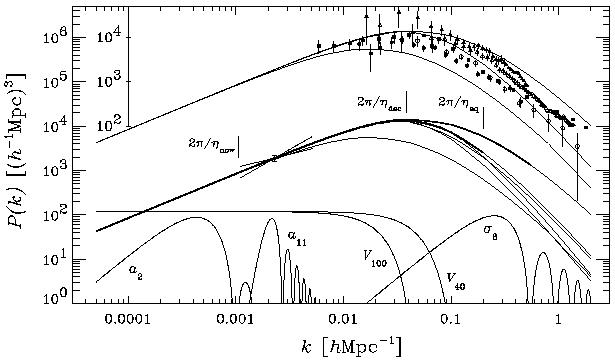
These two CDM variants were identified as the best bets in the COBE interpretation paper (Wright et al. 1992, largely based on Holtzman 1989). In order to discuss them in more detail, it will be best to start by considering the rather complicated but very illuminating Fig. 1.7, showing COBE-normalized linear CHDM and CDM power spectra P (k) compared with four observational estimates of P (k). ⁽⁵⁾ Panel (a) shows the = 1 CHDM models, and Panel (b) shows the CDM models. The heavy solid curves in Panel (a) are for h = 0.5 and _b = 0.05. In the middle section of the figure, the highest of these curves represents the standard CDM model, and the lower ones standard CHDM (N = 1) with = 0.2 (higher) and 0.3; the medium-weight solid curves represent the corresponding CHDM models with two neutrinos equally sharing the same total neutrino mass (N = 2). Note that the N = 2 CHDM power spectra are significantly smaller than those for N = 1 for k 0.04-0.4 h Mpc^-1; this arises because for N = 2 the neutrinos weigh half as much and correspondingly free stream over a longer distance. The result is that N = 2 COBE-normalized CHDM with 0.2 can simultaneously fit the abundance and correlations of clusters (PHKC95, cf. Borgani et al. 1996). The light solid curve is CDM with = h = 0.2.

Figure 1.7. Fluctuation power spectra for COBE-DMR-normalized models: Panel (a) = 1 CDM and CHDM models, Panel (b) 0 + = 1 CDM models. The theoretical spectra are discussed in the text. The data plotted for comparison is squares - real space P (k) from angular APM data (Baugh & Efstathiou 1993), filled circles - estimate of real space P (k) from redshift galaxy and cluster data (Peacock & Dodds 1994), pentagons - IRAS 1.2 Jy redshift space P (k) (Fisher et al. 1993), open and filled triangles - CfA2 and SSRS2 redshift space P (k) (da Costa et al. 1994). At the bottom of each panel are plotted window functions for CMB anisotropy expansion coefficients al (Panel (a): quadrupole a2, and a11; Panel (b) left to right: a2 for 0 = 0.1, 0.3, and 1), bulk flows VR, and the rms mass fluctuation in a sphere of 8h-1 Mpc 8. (From Stompor, Gorski, & Banday 1995, used by permission.)

The ``bow'' superimposed on these curves represents the approximate ``pivot point'' (cf. Gorski et al. 1994) for COBE-normalized ``tilted'' models (i.e., with n_p 1), and the error bar there represents the 1 COBE normalization uncertainty. The window functions for various spherical harmonic coefficients a_l, bulk velocities V_R, and ₈ are shown in the bottom part of this figure (see caption). The bow lies above the a₁₁ window because the statistical weight of the COBE data is greatest for angular wavenumber 11 (cosmic variance is greater for lower , and the ~ 7° resolution of the COBE DMR makes the uncertainty increase for higher ).

The upper section of Panel (a) reproduces the curves for ``standard'' CDM (SCDM, top), = 0.2 N = 1 CHDM, and = 0.2 (light) P (k), compared with several observational P (k) (see caption). Beware of comparing apples to oranges to bananas! Note that the only one of these observational data sets, that of Baugh & Efstathiou (1993, 1994) (squares) is the real-space P (k) reconstructed from the angular APM data; that of Peacock & Dodds (1994) (filled circles) is based on the redshift-space data with a bias-dependent and -dependent correction for redshift distortions and a model-dependent (Peacock & Dodds 1996, Smith et al. 1997) correction for nonlinear evolution; the others are in redshift space. Also, the observations are of galaxies, which are likely to be a biased tracer of the dark matter, while the theoretical spectra are for the dark matter itself. Moreover, as will be discussed in more detail shortly, the real-space linear P (k) are only a good approximation to the true real-space P (k) for k 0.2 h Mpc^-1; nonlinear gravitational clustering makes the actual P (k) rise about an order of magnitude above the linear power spectrum for k 1 h Mpc^-1. Thus one can see that COBE-normalized SCDM predicts a considerably higher P (k) than observations indicate. COBE-normalized = 0.2 CDM predicts a power spectrum shape in better agreement with the data, but with a normalization that is too low. But the P (k) for = 0.2 CHDM, especially with N = 2, is a pretty good fit both in shape and amplitude. The fact that the linear spectrum lies lower than the data for large k is good news for this model, since, as was just mentioned, nonlinear effects will increase the power there.

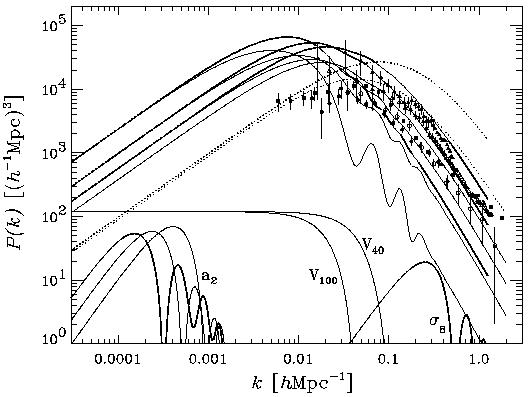
The three heavy solid curves in Panel (b) represent the P (k) for CDM with h = 0.8, _b = 0.02 for ₀ = 0.1 (top, for k = 0.001h Mpc^-1), 0.2, and 0.3 (bottom). The lighter curves are for the same three values of ₀ plus 0.4 (bottom) with h = 0.5, _b = 0.05 (the large wiggles in the latter reflect the effect of the acoustic oscillations with a relatively large fraction of baryons). Dotted curves are for SCDM models with the same pair of h values. The observational P (k) are as in Panel (a).

Note that the power increases at small k as ₀ decreases, with opposite behavior at large k. Also, the COBE-normalized power spectra are unaffected by the value of h for small k, but increase with h for larger k (the fact that the light h = 0.2 curve in Panel (a) is lower than SCDM reflects the same trend). The fact that the data points lie lower than any of the CDM models for k 0.02 is worrisome for the success of CDM, but it is too early to rule out these models on this basis since various effects such as sparse sampling can lead the current observational estimates of P (k) to be too low on large scales (Efstathiou 1996). A better measurement of P (k) on such large scales k 10^-2 h Mpc^-1 will be one of the most important early outputs of the next-generation very large redshift surveys: the 2° field (2DF) survey at the Anglo-Australian Telescope, and the Sloan Digital Sky Survey (SDSS) using a dedicated 2.5 m telescope at the Apache Point Observatory in New Mexico. P (k) is much better determined for larger k by the presently available data, and the fact that the linear ₀ = 0.2 and 0.3 curves lie higher than many of the data points for larger k means that these h = 0.8 models will lie far above the data when nonlinear effects are taken into account. This means that, unless some physical process causes the galaxies to be much less clustered than the dark matter (``anti-biasing''), such models could be acceptable only with a considerable amount of tilt - but that can make the shape of the spectrum fit more poorly.