


In Figure 10, we show an example of the correlation strength, R, and correlation probability, P, between a ZL spectrum and the spectra which result when we assume a range of values (8 × 10⁻⁸ to 1.4 × 10⁻⁷ ergs s-1 cm-2 sr-1 Å-1) for the mean ZL flux contributing to one region of one observed night sky spectrum. Where R and P go to zero, the correct ZL surface brightness has been removed from the observed night sky spectrum.

|
Figure 10. The value of the correlation parameters used to define the strength of the correlation between the residual "airglow" spectrum (the zodiacal light-subtracted night sky spectrum) and the ZL spectrum for different assumed contributions of ZL. The points connected by the dotted line indicate the probability that the two spectra are from the same parent set as a function of the ZL flux assumed. The points connected by the solid line indicate the correlation strength, zero being no correlation. These parameters describe a simple linear correlation as defined in equation 8 (see Press et al. 1992). The ZL surface brightness identified by this method for the observation shown here is 1.08 × 10⁻⁷ ergs s-1 cm-2 sr-1 Å-1. |
The absolute flux of the ZL as measured from each of the 16 spectra
taken on 1995 November 27 and 29 are shown in
Figures 11 -
13. In Figure 11, we
show the average
c( ) as determined
for all 16 spectra over the run for each of the eight spectral
regions. The results are normalized to 1.0 at 4650Å.
This plot illustrates two points: (1) from any single spectral
feature, we find a solution for the ZL flux with a standard deviation
of only 1-6% over 16 individual observations taken on two
nights and independently reduced; and (2), the solution
from independent spectral features are in excellent agreement, and
indicate that the ZL is roughly 5 ± 1% redder than the solar
spectrum, or C(3900, 5100) = 1.05 ± 1 (excluding the point at
~ 4700Å). This color is in excellent agreement with previous
estimates from the ground and space (see
Leinert 1998).
It is also in
excellent agreement with our own measurement of the ZL color from our
simultaneous HST/FOS observations, which give
C(4000, 7000) = 1.044 ± 1 (see Paper I).
) as determined
for all 16 spectra over the run for each of the eight spectral
regions. The results are normalized to 1.0 at 4650Å.
This plot illustrates two points: (1) from any single spectral
feature, we find a solution for the ZL flux with a standard deviation
of only 1-6% over 16 individual observations taken on two
nights and independently reduced; and (2), the solution
from independent spectral features are in excellent agreement, and
indicate that the ZL is roughly 5 ± 1% redder than the solar
spectrum, or C(3900, 5100) = 1.05 ± 1 (excluding the point at
~ 4700Å). This color is in excellent agreement with previous
estimates from the ground and space (see
Leinert 1998).
It is also in
excellent agreement with our own measurement of the ZL color from our
simultaneous HST/FOS observations, which give
C(4000, 7000) = 1.044 ± 1 (see Paper I).

|
Figure 11. The points show
c( |
|
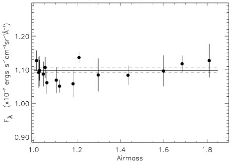
Figure 12. The mean value of the ZL at 4600-4700Å as measured in each of the 16 spectra taken on 1995 November 27 and 29, adopting C(3900, 5100) = 1.05. Each point represent the average of the ZL flux measured in all 8 spectral features in a single observation. The horizontal line shows the mean ZL flux, which is 109.7( ± 0.7) × 10-9 ergs s-1 cm-2 sr-1 Å-1. Dashed lines show the one-sigma statistical error in the mean (0.6%). |
From the solution for the ZL as a function of wavelength we can
explore the impact of the scattered ISL flux on our measurements. If
we increase (decrease) the total flux of the predicted scattered ISL,
Iscat(,
t, , ISL), the
solution for the ZL
decreases (increases) linearly in response; a change of 50% in
the ISL flux corresponds to a change of 6% in the ZL solution at
~ 3950Å, but < 2% at the other wavelengths. Thus, increasing
or decreasing
Iscat(,
t,, ISL) by
50% makes
the ZL solution at 3950Å inconsistent at the two-sigma level with
solutions over the rest of the spectrum for a ZL color of 5 ± 1%.
Also, increasing or decreasing the ISL flux consistently increases the
scatter in the ZL solution at all wavelengths; at 3950Å, the
scatter increases by 40% in response to a change of 50% in the ISL
flux at all airmasses. Although this does not allow us to place a
stronger constraint on the error in
Iscat(,
t,, ISL) than
those discussed in the Appendix, it does provide
independent verification that the predicted
Iscat(,
t,, ISL)
values are in the right range. It also emphasizes that an error of 10% in
Iscat(,
t,, ISL)
changes the mean ZL solution by only 0.4% at 4200-5100Å. As
discussed in the Appendix, the uncertainty in
Iscat(,
t,, ISL)
contributes an
uncertainty to the ZL measurement in Section 6 of
< 0.5% (see Table 1).
, ISL), the
solution for the ZL
decreases (increases) linearly in response; a change of 50% in
the ISL flux corresponds to a change of 6% in the ZL solution at
~ 3950Å, but < 2% at the other wavelengths. Thus, increasing
or decreasing
Iscat(,
t,, ISL) by
50% makes
the ZL solution at 3950Å inconsistent at the two-sigma level with
solutions over the rest of the spectrum for a ZL color of 5 ± 1%.
Also, increasing or decreasing the ISL flux consistently increases the
scatter in the ZL solution at all wavelengths; at 3950Å, the
scatter increases by 40% in response to a change of 50% in the ISL
flux at all airmasses. Although this does not allow us to place a
stronger constraint on the error in
Iscat(,
t,, ISL) than
those discussed in the Appendix, it does provide
independent verification that the predicted
Iscat(,
t,, ISL)
values are in the right range. It also emphasizes that an error of 10% in
Iscat(,
t,, ISL)
changes the mean ZL solution by only 0.4% at 4200-5100Å. As
discussed in the Appendix, the uncertainty in
Iscat(,
t,, ISL)
contributes an
uncertainty to the ZL measurement in Section 6 of
< 0.5% (see Table 1).
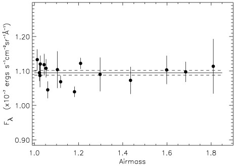
In Figures 12 and 13 we show the mean ZL solution at 4600-4700Å (for C(3900, 5100) = 1.05) as a function of airmass from each of the 16 exposures. Figure 12 shows the solution obtained using all eight spectral features solutions plotted in Figure 11, while Figure 13 shows the solution based on the four spectral features with the smallest standard deviations in Figure 11. The horizontal line in each plot shows the mean, the dashed lines show the one-sigma error in the mean. The difference between the results in the two plots is less than 0.2%. No obvious trends appear in either plot as a function of airmass. In fact, the mean value for points above and below 1.2 airmasses in Figure 13 agrees to better than 0.3% (half of the error in the mean). The error bars in Figure 13 vary from 1-8%, indicative of the small number of measurements (four spectral features) being averaged together to produce the result at each airmass. The standard deviations indicated by the error bars in Figure 12 show less variation from point to point (1.5-5%), as eight measurements contribute to each point.
|
Figure 13. The same as Figure 12, but here only the four features with the smallest error bars have been used to produce the mean value of the ZL at 4600-4700Å in each spectrum The horizontal line shows the mean ZL flux, which is 109.4( ± 0.6) × 10-9 ergs s-1 cm-2 sr-1 Å-1. Dashed lines show the one-sigma statistical error in the mean (0.6%). |
As discussed in the Appendix, we estimate that the uncertainty
in the calculated scattered ZL flux contributes an
uncertainty to the ZL solution of 1.2%. The stability of our ZL
solution with airmass indicates that our calculated net extinction,
which incorperates the ZL scattering models from the Appendix, has the
correct behavior over the night. However there is no way to
independently infer the accuracy of the mean net extinction from the
rms scatter in the ZL solution because the spectral shape of
 eff(, t) does not change
significantly over the
night (see Figure A11); an error in
the mean level of
eff will not
affect the rms scatter in the
solution between exposures. The errors in our result are
summarized in Table 1. We discuss the
systematic uncertainties further in the next section.
eff(, t) does not change
significantly over the
night (see Figure A11); an error in
the mean level of
eff will not
affect the rms scatter in the
solution between exposures. The errors in our result are
summarized in Table 1. We discuss the
systematic uncertainties further in the next section.