5. ANALYSIS

Based on the discussion in the previous section, we can characterize the observed spectrum of the night sky, I_NS, at any time as a combination of airglow, zodiacal light (ZL), diffuse Galactic light (DGL), and scattered interstellar light (ISL) as follows:

(5)

in which _eff(, t) is now the effective extinction for ZL discussed in Section 4 and I_scat(, t,, ISL) is the total scattered ISL flux due to Rayleigh and Mie scattering in the atmosphere.

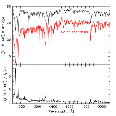
Sharp spectral features are not expected in the EBL because redshifting will blur any distinct spectral features. The EBL will therefore not affect our measurements of the ZL from the strength of the observed Fraunhofer lines. The diffuse Galactic light, which results from scattering of the ambient interstellar radiation field by interstellar dust, is very weak in our field (0.8% of the ZL flux, see Paper I). In addition, as we have already discussed regarding the scattered ISL, the strength of the spectral features we use in our analysis is roughly 1.5 to 3.8 times weaker in the DGL than in the ZL spectrum. The DGL from the target field thus contributes at most 0.2-0.5% percent to the final result (see Figure 7). We subtract this contribution from our ZL measurement after the fact at a level of 0.3%. Emission lines due to ionized gas in the DGL do not contribute in the spectral range of these observations (see Paper I, Martin et al. 1991, Dube et al. 1979, and Reynolds 1990).

Figure 7. In the upper plot, the spectrum of the integrated starlight (ISL) at |b| = 60° is compared to the solar spectrum, which has been scaled to the same flux and offset to allow visual comparison of the spectral features. The lower plot shows the ratio of the two, normalized at 4600Å. Both plots show visually and quantitatively that the absorption lines in the ISL spectrum are weaker than the same features in the solar (and therefore zodiacal light) spectrum.

The observed spectrum can therefore be expressed as the sum of four components: (a) an unstable emission line spectrum, due to airglow; (b) a stable and featureless component, due to EBL; and (c) a stable, absorption line component, due to ZL; and (d) a time variable absorption component due to scattered ISL. The component (c) can be ignored, and (d) has been calculated. The portion of the night sky spectrum which has variable spectral features can therefore be expressed as

(6)

in which I() is the solar spectrum and c() is a scaling factor which relates the mean surface brightness of the ZL to the mean flux of the Sun.

Identifying the appropriate scaling spectrum, c(), is complicated by the fact that the ZL - a pure absorption line spectrum - is greatly obscured by the emission line spectrum of the airglow in the night sky. Airglow features do overlap with some of the solar Fraunhofer lines, as can be seen in the comparison of a night sky spectrum and a scaled solar spectrum shown in Figure 8. The strength of particular airglow lines can vary by several percent during a single night, as can be seen in the comparison of two night sky spectra shown in Figure 9. The airglow spectrum is composed of an effective continuum due to O+NO (NO₂) recombination, broad rotation-vibration transition bands, scattered light, and blended lines, making a continuum level impossible to identify. Not only do rapid temporal variations occur with (de)ionization, but airglow is also a complex function of airmass, observatory location, and local atmospheric conditions such as volcanic activity (van Rhijn 1924, 1925; Roach & Meinel 1955). In short, a stable, fiducial airglow spectrum with meaningful absolute or relative flux cannot be defined. As a result, it is not possible to measure the equivalent width of individual ZL Fraunhofer lines because the ZL continuum level is well hidden. Instead, we have developed a conceptually simple approach to the problem of determining the scaling factors c() which does not involve measuring the equivalent widths explicitly.

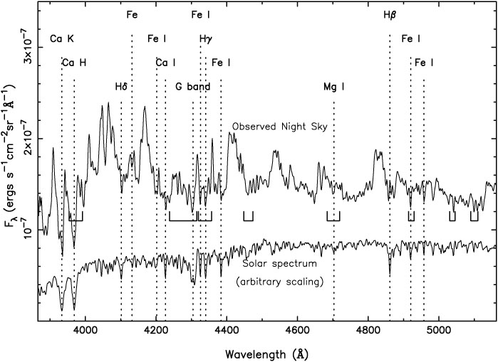
Figure 8. The observed spectrum of the night sky compared to a solar spectrum at arbitrary absolute flux. The solar Fraunhofer absorption lines which are preserved in the ZL are clearly visible in the spectrum of the night sky. The strongest of these lines are marked; several blended solar features are also seen in the night sky spectrum. Square brackets indicate the wavelength regions used in the final analysis.

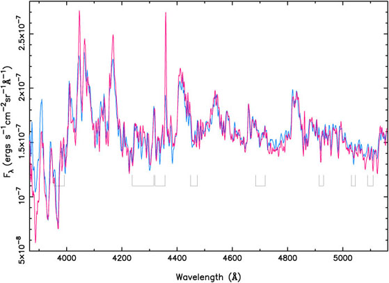
Figure 9. Two spectra of the night sky taken on the same night, several hours from twilight. Rapid fluctuations are evident in the strength of many of the airglow features.

We begin with the assumption that the intrinsic airglow spectrum, time- and airmass-dependent though it may be, does not have spectral features in common with the ZL spectrum. This is borne out by the fact that we get consistent solutions using eight distinct spectral regions spread over 1100Å (see Section 5). When we subtract I_scat(, t,, ISL) and scaled solar spectrum with the correct value for c(), what remains is a pure airglow spectrum, free of solar features:

(7)

We use a linear correlation function to determine when the difference (residual airglow) spectrum is uncorrelated with the solar spectrum and is consequently free of solar features. When the correlation between the difference spectrum and solar spectrum is minimized, the correct ZL surface brightness has been subtracted from the observed night sky.

The only available, high-resolution spectrum of the Sun is the National Solar Observatory Solar Flux Atlas of the integrated solar disk at 0.01Å resolution. The statistical error in the flux calibration of this spectrum is 0.25% as estimated by agreement in overlapping sections of the normalized spectrum. The effects of atmospheric absorption by H₂O or O₂ are negligible below 6500Å, as described in the published Atlas (Kurucz et al. 1984). In the optical, the normalized spectrum can be converted to absolute solar irradiance using the Neckel & Labs (1984) (NL84) absolute calibration. As the NL84 is the standard with respect to which the ZL color is defined, the absolute accuracy of the fiducial solar spectrum is not a source of error in this work. The Solar Flux Atlas, calibrated to NL84, was obtained in digitized form from R.L. Kurucz. It was convolved with a variable width Gaussian to match the resolution of the observed spectra as a function of wavelength. The wavelength-dependent resolution of each program spectrum was determined from the arc lamp spectra which were used for wavelength calibration.

The execution of this method is complicated by the fact that the relative color of the airglow and solar spectra will dominate the strength of the diagnostic correlation if the continuum shapes of both spectra are not properly removed. In order for the strength of the linear correlation of I_air() and I() to reflect the strength of coincident spectral features, both spectra must have stationary mean values as a function of wavelength, as can be seen clearly in the generic expression for a linear correlation:

(8)

In this case, x and y are I_air() and I() respectively, the subscript n runs over wavelength. It is clear from this expression that the mean flux drops out of the correlation, while differences from the mean are crucial.

Of the 47 strongest solar features, we find that 39 give ZL solutions which vary with time by more than 18% over the night. In all cases, this variation is correlated with the strength of adjacent airglow lines. The remaining eight solar features vary by less than 10% with time. The results discussed below are based on these eight spectral regions, indicated in Figures 8 and 9. In these regions, the continuum can be well approximated by a simple second order polynomial fit and easily subtracted, however our results are quite insensitive to the method of continuum fitting. Boxcar smoothing with scales between 75Å and 199Å (at least twice the width of the widest spectral region used in the analysis), second or third order polynomial fitting, and Savitsky-Golay smoothing (Press et al. 1992) all produce identical results.