


Until now we have been discussing the situation in which the experimental result is N events giving precise values x1, ... , xN where the xi may or may not, as the case may be, be all different.
From now on we shall confine our attention to the case
of p measurements (not p events) at the points
x1, ... , xp. The
experimental results are (y1 ±
 1),
... ,(yp ±
p). One such type
of experiment is where each measurement consists of Ni
events.
Then yi = Ni and is
Poisson-distributed with
i =
sqrt[Ni]. In
this case the likelihood function is
1),
... ,(yp ±
p). One such type
of experiment is where each measurement consists of Ni
events.
Then yi = Ni and is
Poisson-distributed with
i =
sqrt[Ni]. In
this case the likelihood function is
|
and
|
We use the notation
 (
( i; x) for the
curve that is to be fitted
to the experimental points. The best-fit curve corresponds to
i =
i*. In this case
of Poisson-distributed points, the
solutions are obtained from the M simultaneous equations
i; x) for the
curve that is to be fitted
to the experimental points. The best-fit curve corresponds to
i =
i*. In this case
of Poisson-distributed points, the
solutions are obtained from the M simultaneous equations
|
If all the Ni >> 1, then it is a good
approximation to
assume each yi is Gaussian-distributed with standard
deviation
i. (It is better
to use  i rather
than Ni for
i2 where
i can
be obtained by integrating
(x)
over the ith interval.) Then
one can use the famous least squares method.
i rather
than Ni for
i2 where
i can
be obtained by integrating
(x)
over the ith interval.) Then
one can use the famous least squares method.
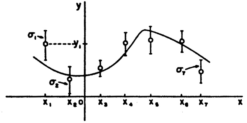
The remainder of this section is devoted to the case in
which yi are Gaussian-distributed with standard
deviations i.
See Fig. 4. We shall now see that the
least-squares method is
mathematically equivalent to the maximum likelihood method. In
this Gaussian case the likelihood function is
| (23) |
where
| (24) |
|
Figure 4.
|
The solutions
i =
i* are given by
minimizing
S() (maximizing
w):

| (25) |
This minimum value of S is called S*, the least squares sum.
The values of i
which minimize are called the least-squares
solutions. Thus the maximum-likelihood and least-squares solutions
are identical. According to Eq. (11), the least-squares
errors are
|
Let us consider the special case in which
(i; x) is
linear in the i:
|
(Do not confuse this f (x) with the f (x) on page 2.)
Then
| (26) |
Differentiating with respect to
j gives
| (27) |
Define
| (28) |
Then
|
In matrix notation the M simultaneous equations giving the least-squares solution are
| (29) |
is the solution for the
*'s. The errors in
are
obtained using Eq. 11. To summarize:
| (30) |
Equation (30) is the complete procedure for calculating the
least squares solutions and their errors. Note that even though
this procedure is called curve-fitting it is never necessary
to plot any curves. Quite often the complete experiment may
be a combination of several experiments in which several different
curves (all functions of the
i) may be jointly
fitted. Then the S-value is the sum over all the points on all the
curves. Note that since
w(*) decreases by
½ unit when one
of the j has the
value (i* ±
 j),
the S-value must increase by one unit. That is,
j),
the S-value must increase by one unit. That is,

|
Example 5 Linear regression with equal errors
(x) is
known to be of the form
(x) =
1 +
2x. There
are p experimental measurements
(yj ±
).Using Eq. (30) we have
|
These are the linear regression formulas which are programmed
into many pocket calculators. They should not be used in
those cases where the
i are not all the
same. If the i
are all equal, the errors
|
or
|
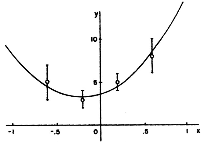
Example 6 Quadratic regression with unequal errors
The curve to be fitted is known to be a parabola. There are four experimental points at x = - 0.6, - 0.2, 0.2, and 0.6. The experimental results are 5 ± 2, 3 ± 1, 5 ± 1, and 8 ± 2. Find the best-fit curve.
|
|
|
|
(x) =
(3.685 ± 0.815) + (3.27 ± 1.96)x + (7.808 ±
4.94)x2 is the
best fit curve. This is shown with the experimental points
in Fig. 5.
|
Figure 5. This parabola is the least squares fit to the 4 experimental points in Example 6. |
Example 7
In example 6 what is the best estimate of y at x = 1? What is the error of this estimate?
Solution: Putting x = 1 into the above equation gives

|
y is obtained using
Eq. 12.
|
Setting x = 1 gives

|
So at x = 1, y = 14.763 ± 5.137.
Least Squares When the yi are Not Independent
Let
|
be the error matrix-of the y measurements. Now we shall treat the more general case where the off diagonal elements need not be zero; i.e., the quantities yi are not independent. We see immediately from Eq. 11a that the log likelihood function is
|
The maximum likelihood solution is found by minimizing
where
| Generalized least squares sum |