


 2DISTRIBUTION
The numerical value of the likelihood function at
 (
( *) can, in principle, be used as
a check on whether one is using the correct type of function for
f (; x). If one is
using the wrong f, the likelihood function will be lower in
height and of greater width. In principle, one can calculate,
using direct probability, the distribution of
(*) assuming a particular true
f (0,
x). Then the probability of getting an
(*) smaller than the value
observed would be a useful
indication of whether the wrong type of function for f had been
used. If for a particular experiment one got the answer that
there was one chance in 104 of getting such a low value of
(*), one would seriously question
either the experiment or the function
f (;x) that
was used.
*) can, in principle, be used as
a check on whether one is using the correct type of function for
f (; x). If one is
using the wrong f, the likelihood function will be lower in
height and of greater width. In principle, one can calculate,
using direct probability, the distribution of
(*) assuming a particular true
f (0,
x). Then the probability of getting an
(*) smaller than the value
observed would be a useful
indication of whether the wrong type of function for f had been
used. If for a particular experiment one got the answer that
there was one chance in 104 of getting such a low value of
(*), one would seriously question
either the experiment or the function
f (;x) that
was used.
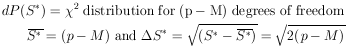
In practice, the determination of the distribution of
(*) is usually an impossibly
difficult numerical integration
in N-dimensional space. However, in the special case of the
least-square problem, the integration limits turn out to be
the radius vector in p-dimensional space. In this case we use
the distribution of
S(*) rather than of
(*). We shall first consider the
distribution of
S(0).
According to Eqs. (23) and (24) the probability element is
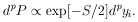
|
Note that S =
 2,
where is the
magnitude of the radius vector
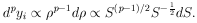
in p-dimensional space. The volume of a p-dimensional sphere
is U
2,
where is the
magnitude of the radius vector
in p-dimensional space. The volume of a p-dimensional sphere
is U  p. The
volume element in this space is then
p. The
volume element in this space is then
|
Thus
|
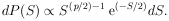
The normalization is obtained by integrating from S = 0 to
S =  .
.
| (30a) |
where
S  S(0).
S(0).
This distribution is the well-known
2 distribution with
p
degrees of freedom. 2
tables of

|
for several degrees of freedom are commonly available - see Appendix V for plots of the above integral.
From the definition of S (Eq. (24)) it is obvious that
 0 = p. One
can show, using Eq. (29) that
0 = p. One
can show, using Eq. (29) that
 = 2p. Hence,
one should be suspicious if his experimental result gives an
S-value much greater than
= 2p. Hence,
one should be suspicious if his experimental result gives an
S-value much greater than

|
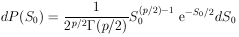
Usually is not known. In
such a case one is interested in the distribution of

|
Fortunately, this distribution is also quite simple. It is
merely the 2
distribution of (p - M) degrees of freedom, where
p is the number of experimental points, and M is the number
of parameters solved for. Thus we haved
| (31) |
Since the derivation of Eq. (31) is somewhat lengthy, it is given in Appendix II.
Example 8
Determine the 2
probability of the solution to Example 6.
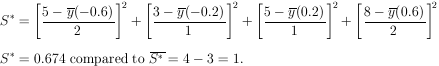
|
According to the 2
table for one degree of freedom the probability of getting
S* > 0.674 is 0.41. Thus the experimental data
are quite consistent with the assumed theoretical shape of
|
Example 9 Combining Experiments
Two different laboratories have measured the lifetime of the K10 to be (1.00 ± 0.01) × 10-10 sec and (1.04 ± 0.02) × 1010 sec respectively. Are these results really inconsistent?
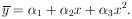
According to Eq. (6) the weighted mean is
* = 1.008 ×
10-10 sec.
(This is also the least squares solution for
 KO.
KO.
Thus

|
According to the 2
table for one degree of freedom, the probability of getting
S* > 3.2 is 0.074. Therefore, according
to statistics, two measurements of the same quantity should be
at least this far apart 7.4% of the time.