4.8. Inflationary "zoology" and the CMB

We have discussed in some detail the generation of fluctuations in inflation, in particular the primordial tensor and scalar power spectra and the relevant parameters A_S, r, and n. We have also looked at one particular choice of potential V() = ⁴ to drive inflation. In fact, pretty much any potential, with suitable fine-tuning of parameters, will work to drive inflation in the early universe. We wish to come up with a classification scheme for different kinds of scalar field potentials and study how we might find observational constraints on one "type" of inflation versus another. Such a "zoology" of potentials is simple to construct. Figure 14 shows three basic types of potentials: large field, where the field is displaced by ~ m_Pl from a stable minimum of a potential, small field, where the field is evolving away from an unstable maximum of a potential, and hybrid, where the field is evolving toward a potential minimum with nonzero vacuum energy.

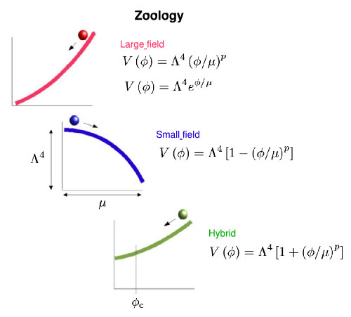Figure 14. A "zoology" of inflation models, grouped into large field, small field, and hybrid potentials.

Large field models are perhaps the simplest types of potentials. These include potentials such as a simple massive scalar field, V() = m^{2 2}, or fields with a quartic self-coupling, V() = ⁴. A general set of large field polynomial potentials can be written in terms of a "height" and a "width" µ as:

(129)

where the particular model is specified by choosing the exponent p. In addition, there is another class of large field potentials which is useful, an exponential potential,

(130)

Small field models are typical of spontaneous symmetry breaking, in which the field is evolving away from an unstable maximum of the potential. In this case, we need not be concerned with the form of the potential far from the maximum, since all the inflation takes place when the field is very close to the top of the hill. As such, a generic potential of this type can be expressed by the first term in a Taylor expansion about the maximum,

(131)

where the exponent p differs from model to model. In the simplest case of spontaneous symmetry breaking with no special symmetries, the leading term will be a mass term, p = 2, and V() = ⁴ - m^{2 2}. Higher order terms are also possible. The third class of models we will call "hybrid", named after models first proposed by Linde [36]. In these models, the field evolves toward the minimum of the potential, but the minimum has a nonzero vacuum energy, V(_min) = ⁴. In such cases, inflation continues forever unless an auxiliary field is added to bring an end to inflation at some point = _c. Here we will treat the effect of this auxiliary field as an additional free parameter. We will consider hybrid models in a similar fashion to large field and small field models,

(132)

Note that potentials of all three types are parameterized in terms of a height ⁴, a width µ, and an exponent p, with an additional parameter _c specifying the end of inflation in hybrid models. This classification of models may seem somewhat arbitrary. ⁽¹¹⁾ It is convenient, however, because the different classes of models cover different regions of the (r, n) plane with no overlap (Fig. 15).

Figure 15. Classes of inflationary potentials plotted on the (r, n) plane.

How well can we constrain these parameters with observation? Figure 8 shows the current observational constraints on the CMB multipole spectrum. As we saw in Sec. 3, the shape of this spectrum depends on a large number of parameters, among them the shape of the primordial power spectrum. However, uncertainties in other parameters such as the baryon density or the redshift of reionization can confound our measurement of the things we are interested in, namely r and n. Figure 16 shows likelihood contours for r and n based on current CMB data [41].

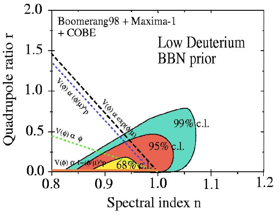Figure 16. Error bars in the r, n plane for the Boomerang and MAXIMA data sets [41]. The lines on the plot show the predictions for various potentials. Similar contours for the most current data can be found in Ref. [20].

Perhaps the most distinguishing feature of this plot is that the error bars are smaller than the plot itself! The favored model is a model with negligible tensor fluctuations and a slightly "red" spectrum, n < 1. Future measurements, in particular the MAP [39] and Planck satellites [40], will provide much more accurate measurements of the C spectrum, and will allow correspondingly more precise determination of cosmological parameters, including r and n. (In fact, by the time this article sees print, the first release of MAP data will have happened.) Figure 17 shows the expected errors on the C spectrum for MAP and Planck, and Fig. 18 shows the corresponding error bars in the (r, n) plane. Note especially that Planck will make it possible to clearly distinguish between different models for inflation.

Figure 17. Expected errors in the C spectrum for the MAP (light blue) and Planck (dark blue) satellites. (Figure courtesy of Wayne Hu [21].)

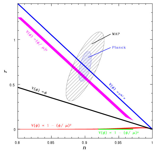Figure 18. Error bars in the r, n plane for MAP and Planck [38]. These ellipses show the expected 2 - errors. The lines on the plot show the predictions for various potentials. Note that these are error bars based on synthetic data: the size of the error bars is meaningful, but not their location on the plot. The best fit point for r and n from real data is likely to be somewhere else on the plot.

¹¹ The classification might also appear ill-defined, but it can be made more rigorous as a set of inequalities between slow roll parameters. Refs. [37 38] contain a more detailed discussion. Back.