


The results available so far may be used as a basis for the determination of the smoothed-out space densities of luminosity and mass, and of the statistical distribution of the masses of galaxies (general field).
The pg luminosity density or the total amount of luminosity in 1 Mpc3 is obtained by a numerical integration based on the curves of Fig. 10 and Fig. 8; the most luminous galaxies make the largest contribution. The result is 1.8 × 10⁸ solar units for the E-So-Ir type group, and 2.3 × 10⁸ solar units for the Sa-Sb-Sc group. The absolute pg magnitude of the sun has been assumed to be +5.37.
The mass density may be derived from the luminosity density, if the mean mass-luminosity ratio can be estimated. The results obtained in 'a previous study by the writer (1964) indicate the following ratios: 22 (E-So), 12 (Sa-Sb), 2.7 (Sc), and 1.2 (Ir I), both masses and luminosities being measured in solar units (for the few Ir II systems a ratio of 10 may be adopted). With the relative frequencies listed in Table 5, the mean ratios for the E-So-Ir and Sa-Sb-Sc groups would be 14 and 5, respectively. Accordingly, the mass density for the first group is 25 × 108, and for the second 12 × 108 solar units. The total density is 37 × 108 solar masses per Mpc3, or 2.5 × 10⁻³¹ gr / cm3 . It should be noted that the density is based on a Hubble parameter H = 80, that it refers to the general field (the mass contributed by the big clusters would however be comparatively small), and that it does not include gas or other dark matter in the intragalactic space. It may be added that in a recent discussion, based on earlier analyses of the observation data available, Peebles and Partridge (1967) have arrived at a mean mass density that is in good agreement with the result found here.
In order to determine the statistical distribution of the masses of all galaxies in a given volume of space, or the mass function, it is necessary to have more detailed information on the luminosity functions corresponding to the separate morphological types. Galaxies of types E-So, Ir I, and Ir II will all be assumed to have the same luminosity function, the curve of Fig. 10 (Fig. 8), with the limitations that the maximum luminosity for Ir I is assumed to be M = -19.5, and for Ir II -20.5, whereas the E-So objects proceed to the upper limit of -22.0; these cut-offs are indicated from studies of the Holmberg (1964) material and the redshift lists. It was found in sect. 12 that the mean magnitude for the Sa-Sb-Sc group is M = -17.7. A detailed study of the present material, combined with the lists mentioned, seems to justify an attempt to subdivide this group. The mean absolute magnitudes are found to be approximately -18.0 (Sa), -18.4 (Sb), -18.0 (Sc - ), and -17.1 (Sc +); with relative frequencies of 6%, 20%, 28%, and 46%, respectively, the weighted mean of the magnitudes will be -17.7. The large increase in relative number from Sa to Sc+ may seem surprising but is indicated by the material at hand. The luminosity function for each spiral type will be assumed to be a normal error-curve, centered on the mean magnitude and with a dispersion of 1.1 magn.; the combined dispersion for all the types will then amount to 1.2 magn., as was found in sect. 12. It should be remarked that the luminosity curve suggested for each of the six type classes is necessarily of an approximate nature, but that the individual deviations may tend to be smoothed out when all the curves are combined.
With rounded-off mass-luminosity ratios of 22 (E-So), 17 (Sa), 10 (Ir II), 9 (Sb), 3 (Sc-), 2 (Sc+), and 1.2 (Ir I), the luminosity curves are transformed into the combined mass distributions for the E-So-Ir and Sa-Sb-Sc groups that are reproduced in Fig. 12 (broken curves). The scale on the ordinate axis gives an absolute calibration, or the logarithmic number per unit of log. mass per Mpc3. The two curves have been adjusted to fit this calibration, that is, the total mass corresponding to each curve agrees with the mass density derived above for the E-So-Ir group and the Sa-Sb-Sc group. The open circles represent the final mass function or the sum of the two curves.
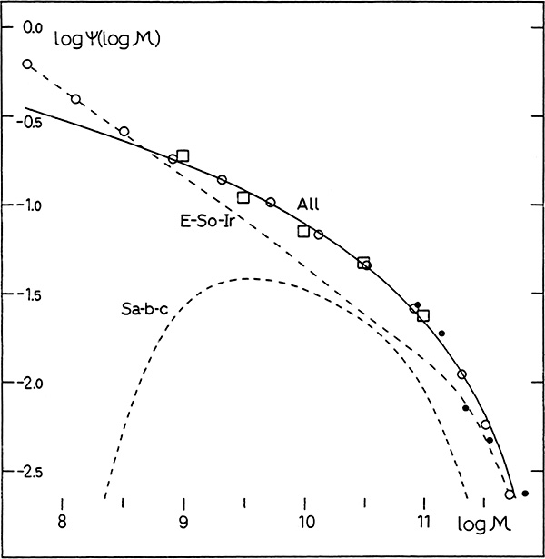 |
Figure 12. Statistical distribution (1 Mpc3) of the log. masses (solar units) of the 274 satellites. The circles give the sum of the distributions corresponding to types E-So-Ir and Sa-Sb-Sc (broken curves). The squares refer to the Local Group and M81 group, and the filled circles to nearby galaxies in the Holmberg (1964) catalogue. The full curve represents the adopted analytical mass function (eq. 5). |
It is found that the final mass function, represented by the full curve in the figure, can be described by a simple analytical expression:
 |
(5) |
which gives the number of galaxies per Mpc3 having masses
referring to a unit interval of
log  . The numerical parameters
have been determined by a least-squares
solution, based on the class frequencies in the interval of log. mass
from 8.9 to 11.3.
The individual frequencies (open circles) show a very good agreement
with this curve.
The only deviations are found for log. masses below 8.5; even for this
interval the curve may possibly approximate to the true mass
distribution, since the mass-luminosity ratios for these dwarf galaxies
have probably been over-estimated. It may be
noted that the parameter within the brackets of eq. (5) has a special
significance, since
it apparently represents the log. maximum mass of galaxies.
. The numerical parameters
have been determined by a least-squares
solution, based on the class frequencies in the interval of log. mass
from 8.9 to 11.3.
The individual frequencies (open circles) show a very good agreement
with this curve.
The only deviations are found for log. masses below 8.5; even for this
interval the curve may possibly approximate to the true mass
distribution, since the mass-luminosity ratios for these dwarf galaxies
have probably been over-estimated. It may be
noted that the parameter within the brackets of eq. (5) has a special
significance, since
it apparently represents the log. maximum mass of galaxies.
In Fig. 12 comparisons have been made with data available from other sources. The squares refer to the Local Group and the M81 group, listed in Table 1. Although the total number of galaxies is small, the successive class frequencies (overlapping means) agree well with the adopted curve. The filled circles represent the most massive galaxies in the Holmberg (1964) list, which is apparently complete, as regards galaxies with log. masses larger than 10.8 (total number = 54). Even in this case, there is a good agreement with the full curve.
The mass function can be presented in a different way, which maybe of
interest from a cosmological point of view. The curve of
Fig. 13 represents the function
×
 () or the total mass of all
galaxies in 1 Mpc3 that have masses referring to a
unit interval of
. If all galaxies were
formed directly from the primeval gas, as is
usually postulated, the curve would describe an. important feature of
the original condensation process, that is, it would show the total
amount of gas that went into the
formation of galaxies of different mass. As is easily proved, the
statistical distribution of galaxian masses,
() , is equal to the function
() or the total mass of all
galaxies in 1 Mpc3 that have masses referring to a
unit interval of
. If all galaxies were
formed directly from the primeval gas, as is
usually postulated, the curve would describe an. important feature of
the original condensation process, that is, it would show the total
amount of gas that went into the
formation of galaxies of different mass. As is easily proved, the
statistical distribution of galaxian masses,
() , is equal to the function
 (log
) , multiplied by the factor
log e / ;
accordingly, the function
×
() will be equal to
0.0078(12.1 - log
)2 .
An integration of this function leads to 37 × 108 solar
units, or the mass density that
was derived above. We find that galaxies with log. masses above 11.0
contribute
about 46 o/o of the total mass in a given volume of space, and that
galaxies with log. masses in the intervals 10-11 and 9-10 represent 40
o/o and 11 o/o, respectively.
The contribution by galaxies with masses below 109 solar
units is so small, less
than 3 o/o, that it may be neglected. These figures refer to the general
field, but an inclusion of the big clusters of galaxies would presumably
not change the results to any great extent.
(log
) , multiplied by the factor
log e / ;
accordingly, the function
×
() will be equal to
0.0078(12.1 - log
)2 .
An integration of this function leads to 37 × 108 solar
units, or the mass density that
was derived above. We find that galaxies with log. masses above 11.0
contribute
about 46 o/o of the total mass in a given volume of space, and that
galaxies with log. masses in the intervals 10-11 and 9-10 represent 40
o/o and 11 o/o, respectively.
The contribution by galaxies with masses below 109 solar
units is so small, less
than 3 o/o, that it may be neglected. These figures refer to the general
field, but an inclusion of the big clusters of galaxies would presumably
not change the results to any great extent.
 |
Figure 13. The mass function presented in a different way. The curve gives the total mass of all galaxies in 1 Mpc3 that have masses referring to a unit interval of mass. |
In conclusion, it may be added that there is an unexpected agreement
between the mass function for galaxies and the mass function for
stars. It seems possible to
describe the initial stellar-mass function, as derived by
Limber (1960),
by an analytical expression of the same type as that given in eq. (5). A
least-squares solution,
based on the frequencies of log. stellar masses in the interval 0.0 to
+2.0, gives a distribution = const.(2.5 - log
)2 . The
numerical parameter within the brackets
may also in this case represent the maximum log. mass of the initial gas
cloud (although condensations of this size do not give birth to stable
stars). It is an interesting question whether this agreement is a
coincidence or whether it may be interpreted as indicating that the
condensation processes leading to the formation of galaxies and of stars
both follow the same general law.
| NGC | Class | Type |  CN
CN |
m - M | Nobs | Nphys |
| 24 | A | Sc - | - | 29.5 | 4 | + 1 |
| 224 | A | Sb - | +0.07 | 24.18 | 2 | + 2 |
| 247 | A | Sc + | - | 28.0 | 6 | + 4 |
| 253 | A | Sc | - | 28.0 | 1 | 0 |
| 598 | B | Sc + | +0.13 | 24.18 | 0 | 0 |
| 628 | B | Sc - | +0.01 | 29.7 | 8 | + 5 |
| 672 | C | Sc + | -0.09 | 28.7 | 7 | + 5 |
| 784 | A | Sc + | - | 28.7 | 2 | + 1 |
| 891 | A | Sb + | - | 29.4 | 6 | + 4 |
| 908 | A | Sc - | +0.14 | 30.8 | 2 | 0 |
| 925 | B | Sc + | -0.11 | 29.4 | 2 | - 1 |
| 936 | B | So | +0.04 | 30.8 | 12 | - |
| 1003 | A | Sc + | -0.09 | 29.4 | 13 | - |
| 1023 | A | So | 0.00 | 29.4 | 5 | + 3 |
| 1042 | C | Sc - | +0.06 | 30.2 | 8 | + 5 |
| 1055 | C | Sb + | +0.01 | 28.0 | 6 | + 5 |
| 1058 | B | Sc - | -0.12 | 29.4 | 10 | - |
| 1090 | C | Sb + | -0.15 | 28.9 | 7 | + 5 |
| 1232 | B | Sc - | +0.18 | 30.7 | 2 | - 1 |
| 1300 | B | Sb + | -0.01 | 30.9 | 3 | 0 |
| 1325 | C | Sb + | -0.07 | 31.0 | 5 | + 2 |
| 1337 | A | Sc + | +0.21 | 29.3 | 1 | - 2 |
| 1507 | A | Sc | - | 30.1 | 2 | - 1 |
| 1560 | A | Sc + | - | 28.0 | 2 | 0 |
| 1637 | B | Sc - | +0.14 | 29.5 | 3 | 0 |
| 1784 | B | Sc - | +0.19 | 29.8 | 4 | + 1 |
| 2146 | B | Sc - | - | 30.1 | 7 | + 4 |
| 2403 | A | Sc + | -0.04 | 27.60 | 6 | + 5 |
| 2541 | A | Sc + | -0.04 | 29.0 | 1 | 0 |
| 2613 | A | Sb | - | 31.2 | 6 | + 2 |
| 2681 | B | Sa | -0.17 | 30.9 | 5 | + 2 |
| 2683 | A | Sb - | -0.07 | 29.8 | 2 | 0 |
| 2685 | B | So | 0.00 | 30.4 | 5 | + 2 |
| 2715 | A | Sc - | -0.04 | 30.8 | 4 | + 2 |
| 2835 | B | Sc - | - | 29.5 | 1 | - 2 |
| 2841 | A | Sb - | -0.03 | 30.1 | 9 | - |
| 2903 | B | Sc - | -0.03 | 29.5 | 3 | 0 |
| 3003 | A | Sc | - | 30.2 | 2 | 0 |
| 3027 | C | Sc + | - | 30.1 | 5 | + 2 |
| 3031 | C | Sb - | 0.00 | 27.30 | 8 | + 7 |
| 3044 | A | Sc | - | 30.8 | 6 | + 3 |
| 3079 | A | Sc - | - | 30.2 | 3 | 0 |
| 3166 | C | Sa | -0.06 | 31.0 | 6 | + 3 |
| 3184 | B | Sc - | +0.08 | 29.3 | 1 | - 2 |
| 3190 | C | Sa | -0.04 | 30.8 | 7 | + 4 |
| 3198 | A | Sc - | +0.14 | 29.1 | 2 | + 1 |
| 3227 | C | Sb | - | 30.5 | 7 | + 4 |
| 3239 | B | Sc + | - | 29.9 | 10 | - |
| 3254 | A | Sb + | - | 30.8 | 1 | - 1 |
| 3301 | A | So | - | 31.0 | 4 | + l |
| 3310 | B | Sb + | - | 30.7 | 2 | - 1 |
| 3319 | A | Sc + | -0.05 | 29.3 | 3 | 0 |
| 3338 | B | Sc - | +0.24 | 29.8 | 7 | + 4 |
| 3344 | B | Sc - | +0.03 | 29.6 | 6 | + 3 |
| 3351 | B | Sb + | 0.00 | 29.8 | 1 | - 2 |
| 3359 | B | SC + | -0.11 | 30.2 | 7 | + 4 |
| 3368 | B | Sa | +0.02 | 29.8 | 1 | - 2 |
| 3384 | C | So | - | 29.7 | 6 | + 3 |
| 3423 | B | Sc + | +0.14 | 29.8 | 5 | + 2 |
| 3432 | A | Sc + | -0.12 | 29.8 | 5 | - 1 |
| 3447 | B | Sc + | - | 30.1 | 7 | + 4 |
| 3486 | B | So - | +0.09 | 29.6 | 4 | + 1 |
| 3495 | A | Sc | - | 30.1 | 6 | + 2 |
| 3510 | A | Sc | - | 29.6 | 5 | + 3 |
| 3511 | C | Sc | - | 30.4 | 2 | - 1 |
| 3521 | A | Sb - | +0.01 | 29.2 | 8 | + 5 |
| 3556 | A | SC + | - | 29.6 | 7 | + 2 |
| 3623 | C | Sa | -0.06 | 29.8 | 2 | - 1 |
| 3627 | C | Sb + | -0.02 | 29.8 | 2 | - 1 |
| 3628 | C | Sb + | - | 29.8 | 5 | + 2 |
| 3631 | B | Sc - | -0.23 | 30.6 | 3 | 0 |
| 3642 | B | SC - | -0.10 | 30.3 | 7 | + 4 |
| 3675 | A | Sb - | - | 29.8 | 1 | - 1 |
| 3726 | B | So - | -0.11 | 30.3 | 6 | + 3 |
| 3756 | C | Sc - | 0.00 | 30.4 | 6 | + 3 |
| 3810 | B | Sc - | +0.10 | 29.8 | 12 | - |
| 3893 | B | Sc - | - | 30.6 | 5 | + 2 |
| 3898 | B | Sa | - | 30.8 | 7 | + 4 |
| 3938 | B | SC - | +0.07 | 30.8 | 7 | + 4 |
| 3953 | B | Sb + | -0.01 | 30.2 | 8 | + 5 |
| 3992 | B | Sb + | +0.18 | 30.2 | 9 | - |
| 4026 | A | So | - | 30.4 | 3 | 0 |
| 4051 | B | Sb + | -0.11 | 30.1 | 2 | - 1 |
| 4064 | A | Sa | - | 30.4 | 5 | + 2 |
| 4088 | A | Sc - | 0.00 | 31.0 | 6 | + 4 |
| 4096 | A | Sc + | +0.13 | 30.3 | 1 | - 1 |
| 4111 | C | So | -0.07 | 30.2 | 11 | - |
| 4116 | C | Sc + | +0.03 | 30.5 | 3 | 0 |
| 4123 | C | Sc - | +0.03 | 30.5 | 3 | 0 |
| 4151 | B | Sa | - | 30.5 | 8 | + 5 |
| 4178 | A | Sc + | +0.11 | 30.5 | 2 | 0 |
| 4192 | A | Sb + | +0.05 | 30.2 | 6 | + 3 |
| 4206 | C | Sc - | - | 29.7 | 11 | - |
| 4216 | A | Sb - | +0.11 | 29.7 | 11 | - |
| 4235 | C | Sa | +0.06 | 30.5 | 8 | + 5 |
| 4236 | A | Sc + | - | 25.9 | 5 | + 3 |
| 4242 | B | Sc + | 0.00 | 29.5 | 2 | - 1 |
| 4244 | C | Sc + | - | 27.1 | 0 | - 1 |
| 4254 | B | Sc - | +0.07 | 30.5 | 1 | - 2 |
| 4258 | A | Sb + | -0.09 | 29.0 | 7 | + 4 |
| 4274 | C | Sa | +0.09 | 30.0 | 7 | + 4 |
| 4293 | A | Sa | - | 29.7 | 2 | 0 |
| 4298 | C | Sc - | +0.06 | 30.5 | 4 | + 1 |
| 4302 | C | S | - | 30.5 | 6 | + 3 |
| 4303 | C | Sc - | +0.06 | 30.5 | 5 | + 2 |
| 4314 | B | Sa | - | 30.2 | 5 | + 2 |
| 4321 | B | Sc - | -0.13 | 30.5 | 7 | + 4 |
| 4371 | B | S | -0.01 | 30.5 | 9 | - |
| 4374 | C | So | +0.02 | 30.5 | 8 | + 5 |
| 4382 | C | So | -0.01 | 30.5 | 3 | 0 |
| 4395 | B | Sc + | 0.00 | 27.1 | 0 | - 1 |
| 4414 | B | Sc - | - | 29.8 | 13 | - |
| 4429 | B | So | +0.07 | 30.5 | 2 | - 1 |
| 4442 | C | So | -0.02 | 30.5 | 11 | - |
| 4448 | A | Sb - | - | 29.7 | 9 | - |
| 4450 | B | Sb - | +0.04 | 30.5 | 4 | + 1 |
| 4490 | C | Sc + | -0.09 | 30.5 | 2 | - 1 |
| 4496 | C | Sc + | 30.5 | 4 | + 1 | |
| 4501 | B | Sb + | +0.12 | 30.5 | 2 | - 1 |
| 4517 | A | Sc - | - | 29.7 | 4 | + 2 |
| 4527 | A | Sb - | +0.13 | 30.5 | 2 | - 1 |
| 4535 | B | Sc - | +0.02 | 30.5 | 6 | + 3 |
| 4536 | A | Sc - | +0.10 | 30.5 | 5 | + 3 |
| 4548 | B | Sb + | -0.03 | 30.5 | 3 | 0 |
| 4559 | B | Sc + | +0.19 | 29.7 | 3 | 0 |
| 4565 | A | Sb + | - | 29.4 | 6 | + 2 |
| 4567 | C | Sc - | - | 30.5 | 8 | + 5 |
| 4568 | C | Sc - | - | 30.5 | 8 | + 5 |
| 4569 | A | Sb + | -0.17 | 30.5 | 5 | + 1 |
| 4571 | B | Sc + | +0.23 | 30.5 | 2 | - 1 |
| 4579 | B | Sb - | -0.02 | 30.5 | 3 | 0 |
| 4586 | C | Sa | +0.22 | 30.5 | 4 | + 1 |
| 4594 | A | Sa | +0.11 | 30.5 | 3 | - 1 |
| 4596 | C | Sa | +0.10 | 30.5 | 3 | 0 |
| 4618 | C | Sc + | -0.15 | 30.4 | 5 | + 2 |
| 4631 | C | So + | - | 28.6 | 7 | + 5 |
| 4651 | B | Sc - | -0.02 | 30.5 | 4 | + 1 |
| 4654 | C | Sc - | +0.11 | 30.5 | 5 | + 2 |
| 4665 | B | So | - | 30.5 | 1 | - 2 |
| 4666 | A | Sc - | +0.01 | 30.5 | 5 | + 3 |
| 4689 | B | Sc - | +0.03 | 30.5 | 3 | 0 |
| 4698 | B | Sa | -0.01 | 30.5 | 2 | - 1 |
| 4710 | A | So | - | 30.6 | 1 | - 1 |
| 4725 | B | Sb + | -0.03 | 30.2 | 5 | + 2 |
| 4736 | B | Sb - | 29.4 | 2 | - 1 | |
| 4754 | C | So | - | 30.8 | 2 | - 1 |
| 4762 | C | So | - | 30.8 | 2 | - 1 |
| 4781 | C | Sc + | - | 29.9 | 4 | + 1 |
| 4826 | B | Sb - | +0.07 | 29.9 | 1 | - 2 |
| 4856 | A | Sa | - | 30.5 | 7 | + 3 |
| 4941 | B | Sb - | - | 30.5 | 4 | + 1 |
| 5033 | C | Sc - | +0.02 | 29.3 | 3 | 0 |
| 5055 | B | Sb + | -0.11 | 29.3 | 5 | + 2 |
| 5194 | C | Sc - | - | 29.8 | 3 | 0 |
| 5204 | A | Sc + | -0.11 | 29.1 | 5 | + 2 |
| 5364 | C | Sc - | +0.24 | 30.0 | 3 | 0 |
| 5457 | C | Sc - | 0.00 | 27.7 | 7 | + 6 |
| 5474 | C | Sc + | -0.04 | 29.1 | 1 | - 1 |
| 5585 | B | Sc + | -0.04 | 29.1 | 0 | - 2 |
| 5746 | A | Sb - | +0.11 | 31.2 | 5 | + 2 |
| 5775 | C | Sb + | - | 31.0 | 8 | + 5 |
| 5866 | A | So | - | 30.4 | 5 | + 1 |
| 5879 | A | Sb + | - | 30.6 | 2 | - 1 |
| 5907 | A | Sb + | - | 29.0 | 4 | + 1 |
| 6015 | A | Sc + | +0.20 | 30.6 | 0 | - 2 |
| 6503 | A | Sc - | -0.14 | 29.6 | 3 | + 1 |
| 7331 | A | Sb + | -0.09 | 30.2 | 7 | + 4 |
| 7361 | A | Sc | - | 30.9 | 1 | - 1 |
| 7640 | A | Sc + | - | 29.2 | 0 | - 1 |
| 7741 | B | Sc + | -0.08 | 30.2 | 6 | + 3 |
| 7814 | A | Sa | - | 31.0 | 6 | + 3 |
| 239* | B | Sc - | -0.13 | 30.3 | 3 | 0 |
| A 103 | B | Sc + | - | 30.6 | 6 | + 3 |
| Rh 80 | C | Sc + | - | 29.7 | 3 | 0 |