13.3.5. Variability

Nearly all compact radio sources, when observed over a sufficient period of time and with sufficient precision, show variability on time scales ranging from a few days to a few years and with fractional flux density changes ranging from a few percent to about 100 percent. The most rapid variations occur in BL Lac objects. In general, the observed variations may be described as outbursts which are strongest at the highest frequencies and propagate toward lower frequencies with reduced amplitude (Figure 13.5) (e.g., Dent et al. 1974, Dent and Kapitsky 1976, Altschuler and Wardle 1977, Andrew et al. 1978, Fanti et al. 1981, 1983, Epstein et al. 1982, Aller et al. 1985). However, the variations which are observed at frequencies less than 1 GHz or so for the most part appear unrelated to those observed at centimeter wavelengths and, as discussed below, are probably due to a different phenomenon.

Figure 13.5. Variations in the flux density of the quasar 3C454.3 observed over a wide range of wavelengths. [Data taken from Aller et al. (1985); Altschuler and Wardle (1977), with permission from the Royal Astronomical Society; and Pauliny-Toth et al. (1987). Reprinted by permission from Nature, Vol. 328, No. 6133, pp 778. Copyright(c) 1987, Macmillan Magazines Ltd.]

The observation of variations in polarization is difficult since the degree of linear polarization is typically only a few percent, and the time scale for significant changes appears to be more rapid than for variations in total flux density (e.g., Aller et al. 1985). There appears to be no clear pattern to the variations in observed polarization. In some sources, there is a preferred orientation and the position angle remains constant throughout several flux density outbursts; in others, the direction may change even in the absence of obvious changes in total intensity.

Except for the most rapid variations, it is convenient to discuss the observed variations in terms of an expanding cloud of relativistic particles which is initially opaque out to short wavelengths but which becomes optically thin at successively longer wavelengths. In its. simplest form, the model assumes that the relativistic particles are homogeneously distributed, that they initially have a power law spectrum, that they are produced in a very short time, in a small space, that the subsequent expansion occurs in three dimensions at a constant velocity, and that during the expansion the magnetic flux is conserved. Thus ₂ / ₁ = t₂ / t₁, and B₂ / B₁ = (₁ / ₂)² = (t₁ / t₂)², where is the angular size, t the elapsed time since the outburst, B the magnetic field, and the subscripts 1 and 2 refer to measurements made at epochs t₁ and t₂. The discussion below follows that of Kellermann and Pauliny-Toth (1968) and van der Laan (1966), and is based on ideas first described by Shklovsky (1965).

The observed flux density as a function of frequency, , and time, t, is shown in Figure 13.6 and is described by

(13.24)

where S_m1 is the maximum flux reached at frequency _m1 at time t₁.

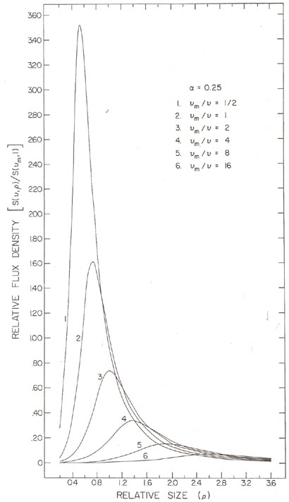Figure 13.6. Variation in flux density and frequency for adiabatically expanding homogeneous source (van der Laan, 1966. Reprinted by permission from Nature, Vol. 211, No. 5054, pp. 1131. Copyright(c) 1966. Macmillan Magazines Ltd.)

If the optical depth, , is taken as the value at the frequency, _m at which the flux density is a maximum, then it is given by the solution of

(13.25)

The maximum flux density at a given frequency as a function of time occurs at a different optical depth, _t, given by the solution of

(13.26)

In the region of the spectrum where the source is opaque ( >> 1), the flux density increases with time as S₂ / S₁ = (t₂ / t₁)³. Where it is transparent ( << 1), the flux density decreases as S₂ / S₁ = (t₂ / t₁)^-2.

The frequency, _m, at which the intensity is a maximum is given by

(13.27)

and the maximum flux density, S_m, at that frequency is given by

(13.28)

Quantitative comparison with observations is difficult since most sources have multiple outbursts which overlap in frequency and time (e.g., Figure 13.6). Moreover, while a homogeneous, isotropic, flux-conserving model with constant expansion velocity is mathematically simple, more realistic models must consider nonconstant expansion rates, nonconservation of magnetic flux, changes in the electron energy index, p, the finite acceleration time for the relativistic particles, the inhomogeneous distribution of relativistic plasma, and the initial finite dimensions. In those few cases where individual outbursts may be isolated, the observed variations qualitatively conform to the simple model, with S_m, t_m, and _m described by Equations (13.27) and (13.28) with 1 p < 1.5. In general, however, the observed variations at the lower frequencies are larger than expected from an adiabatically expanding source, and it appears to be necessary to include the effect of continued particle injection or acceleration (e.g., Peterson and Dent 1973). Models which consider expansion along only one dimension, as expected from a jet, may also be more realistic than a spherical expansion.

Because the source dimensions are initially finite, the initial spectrum is always transparent at frequencies higher than some critical frequency, ₀. Above this frequency, the flux density variations occur simultaneously at all frequencies and reflect only the rate of relativistic particle production or decay due to synchrotron and inverse Compton radiation losses. Characteristically, ₀ is in the range of 10 to 30 GHz. From Equation (13.18) this gives an initial size of ~ 10^-3 arcseconds for B ~ 1 gauss, corresponding to linear sizes of a few parsecs at z ~ 1. In those sources where good data exist in the spectral region v > ₀, the observed variations occur with roughly equal amplitude at all frequencies, indicating an initial spectral index ~ 0, or p ~ 1, in reasonable agreement with the value of p derived from Equation (13.27) or (13.28).

The greatest theoretical difficulty in interpreting the observations of variable compact radio sources in terms of conventional synchrotron models comes from the excessively high brightness temperatures implied from the observations of rapid variations. The problem arises because causality arguments require that if variability is observed on a time scale , then the dimensions of the radiating region must be less than c, since otherwise differential signal travel time over the source would blur any variations. Using the distance obtained from the redshift, z, an upper limit to the angular size, , may be calculated. This value of often leads to brightness temperatures well in excess of 10¹² K, in apparent conflict with the maximum value allowed for an incoherent synchrotron source, particularly for variability observed at frequencies < 1 GHz or on time scales t << 1 year (e.g., Jones and Burbidge 1973).

For some years the variability observed at very low frequencies aroused considerable speculation about the reality of the observations, or about the validity of accepting quasar redshifts as a measure of distance. It now appears, however, that the low-frequency variations are most easily interpreted as the result of scintillations in the ionized interstellar medium (Shapirovskaya 1978, Rickett et al. 1984). The very rapid variations observed at centimeter wavelengths, with time scales of the order of one day (Heeschen 1984), are probably also unrelated to the "classical" variability and may also be due to the same scintillation phenomenon (Blandford et al. 1986).

However, causality arguments applied to the variations which occur on time scales of the order of one year at centimeter wavelengths also predict apparent brightness temperatures which often exceed the inverse Compton limit by a factor of 10 to 100, as well as an X-ray flux which is many orders of magnitude above the values actually observed. Shortly after the implication of inverse Compton scattering was first appreciated (e.g., Hoyle et al. 1966), it was realized that the problem could be avoided if the source of radiation was moving toward the observer with a velocity close to the speed of light (Rees 1966). In this case, the apparent time scale seen by an observer at rest is shortened and the apparent brightness temperature is enhanced by "Doppler boosting." Support for the so-called "relativistic beaming" model comes from the very long baseline (VLBI) observations of "superluminal" radio sources discussed in Section 13.3.7.