Copyright © 2002 by Annual Reviews. All rights reserved
| Annu. Rev. Astron. Astrophys. 2002. 40:
171-216 Copyright © 2002 by Annual Reviews. All rights reserved |


2.1. Standard Cosmological Paradigm
While a review of the standard cosmological paradigm is not our intention (see [Narkilar & Padmanabhan, 2001] for a critical appraisal), we briefly introduce the observables necessary to parameterize it.
The expansion of the Universe is described by the scale
factor a(t), set to unity today, and by the current
expansion rate,
the Hubble constant H0 = 100h km
sec-1 Mpc-1, with
h  0.7
[Freedman et al, 2001].
The Universe is flat (no spatial curvature) if the total
density is equal to the critical density,
0.7
[Freedman et al, 2001].
The Universe is flat (no spatial curvature) if the total
density is equal to the critical density,
 c =
1.88h2 × 10-29 g cm-3; it
is open (negative
curvature) if the density is less than this and closed (positive
curvature) if greater.
The mean densities of different components of the
Universe control a(t) and are typically expressed today in
units of the critical density
c =
1.88h2 × 10-29 g cm-3; it
is open (negative
curvature) if the density is less than this and closed (positive
curvature) if greater.
The mean densities of different components of the
Universe control a(t) and are typically expressed today in
units of the critical density
 i, with
an evolution with a specified by equations of state
wi = pi /
i,
where pi is the pressure of the ith
component. Density fluctuations
are determined by these parameters through the gravitational instability of
an initial spectrum of fluctuations.
i, with
an evolution with a specified by equations of state
wi = pi /
i,
where pi is the pressure of the ith
component. Density fluctuations
are determined by these parameters through the gravitational instability of
an initial spectrum of fluctuations.
The working cosmological model contains photons, neutrinos, baryons,
cold dark matter and dark energy with densities proscribed within
a relatively tight range. For the radiation,
r = 4.17
× 10-5h-2 (wr =
1/3). The photon contribution to the radiation is determined to high
precision by the measured CMB temperature,
T = 2.728 ± 0.004K
[Fixsen et al, 1996].
The neutrino contribution follows from the assumption of 3 neutrino
species, a standard thermal history, and a negligible mass
m <<
1eV. Massive neutrinos have an equation of state
w = 1/3
<<
1eV. Massive neutrinos have an equation of state
w = 1/3
 0 as the particles
become non-relativistic. For
m ~ 1eV this
occurs at
a ~ 10-3 and can leave a small but potentially measurable
effect on the CMB anisotropies
[Ma & Bertschinger, 1995,
Dodelson et al, 1996].
0 as the particles
become non-relativistic. For
m ~ 1eV this
occurs at
a ~ 10-3 and can leave a small but potentially measurable
effect on the CMB anisotropies
[Ma & Bertschinger, 1995,
Dodelson et al, 1996].
For the ordinary matter or baryons,
b
 0.02
h-2 (wb
0)
with statistical uncertainties at about the ten percent level determined
through studies of the light element abundances
(for reviews, see
[Boesgaard & Steigman, 1985,
Schramm & Turner, 1998,
Tytler et al, 2000]).
This value is in strikingly good agreement with that implied by the
CMB anisotropies themselves as we shall see.
There is very strong evidence that there is also
substantial non-baryonic dark matter.
This dark matter must be close to cold (wm = 0) for
the gravitational instability paradigm to work
[Peebles, 1982]
and when added to the baryons gives a total in non-relativistic matter of
m
1/3.
Since the Universe appears to be flat, the total
tot must
be equal to one. Thus, there
is a missing component to the inventory, dubbed dark energy, with
0.02
h-2 (wb
0)
with statistical uncertainties at about the ten percent level determined
through studies of the light element abundances
(for reviews, see
[Boesgaard & Steigman, 1985,
Schramm & Turner, 1998,
Tytler et al, 2000]).
This value is in strikingly good agreement with that implied by the
CMB anisotropies themselves as we shall see.
There is very strong evidence that there is also
substantial non-baryonic dark matter.
This dark matter must be close to cold (wm = 0) for
the gravitational instability paradigm to work
[Peebles, 1982]
and when added to the baryons gives a total in non-relativistic matter of
m
1/3.
Since the Universe appears to be flat, the total
tot must
be equal to one. Thus, there
is a missing component to the inventory, dubbed dark energy, with
 2/3.
The cosmological constant
(w = - 1)
is only one of several possible candidates but we will generally assume
this form unless otherwise specified.
Measurements of an accelerated expansion from distant supernovae
[Riess et al, 1998,
Perlmutter et al, 1999]
provide entirely independent evidence for dark energy in this amount.
2/3.
The cosmological constant
(w = - 1)
is only one of several possible candidates but we will generally assume
this form unless otherwise specified.
Measurements of an accelerated expansion from distant supernovae
[Riess et al, 1998,
Perlmutter et al, 1999]
provide entirely independent evidence for dark energy in this amount.
The initial spectrum of density
perturbations is assumed to be a power law with
a power law index or tilt of
n 1 corresponding
to a scale-invariant spectrum.
Likewise the initial spectrum of gravitational
waves is assumed to be scale-invariant, with an amplitude parameterized
by the energy scale of inflation Ei,
and constrained to be small compared with the initial density spectrum.
Finally the formation of structure
will eventually reionize the Universe at some redshift
7  zri
20.
zri
20.
Many of the features of the anisotropies will be produced even if these parameters fall outside the expected range or even if the standard paradigm is incorrect. Where appropriate, we will try to point these out.
The basic observable of the CMB is its intensity
as a function of frequency and direction on the sky
 .
Since the CMB spectrum is an extremely good blackbody
[Fixsen et al, 1996]
with a nearly constant temperature across the sky T, we generally
describe this observable in terms of a temperature fluctuation
.
Since the CMB spectrum is an extremely good blackbody
[Fixsen et al, 1996]
with a nearly constant temperature across the sky T, we generally
describe this observable in terms of a temperature fluctuation
 () =
() =
 T / T.
If these fluctuations are Gaussian, then the multipole moments of the temperature field
 |
(1) |
are fully characterized by their power spectrum
 |
(2) |
whose values as a function of
 are independent in a given
realization.
For this reason predictions and analyses are typically performed
in harmonic space. On small sections of the sky where its curvature
can be neglected, the spherical harmonic analysis becomes ordinary
Fourier analysis in two dimensions. In this limit
becomes the Fourier
wavenumber. Since the angular wavelength
are independent in a given
realization.
For this reason predictions and analyses are typically performed
in harmonic space. On small sections of the sky where its curvature
can be neglected, the spherical harmonic analysis becomes ordinary
Fourier analysis in two dimensions. In this limit
becomes the Fourier
wavenumber. Since the angular wavelength
 =
2
=
2 /
, large multipole moments
corresponds to small angular scales with
~ 102 representing
degree scale separations. Likewise, since in this limit
the variance of the field is
/
, large multipole moments
corresponds to small angular scales with
~ 102 representing
degree scale separations. Likewise, since in this limit
the variance of the field is
 d2
C /
(2)2, the
power spectrum is usually displayed as
d2
C /
(2)2, the
power spectrum is usually displayed as
 |
(3) |
the power per logarithmic interval in wavenumber for
>> 1.
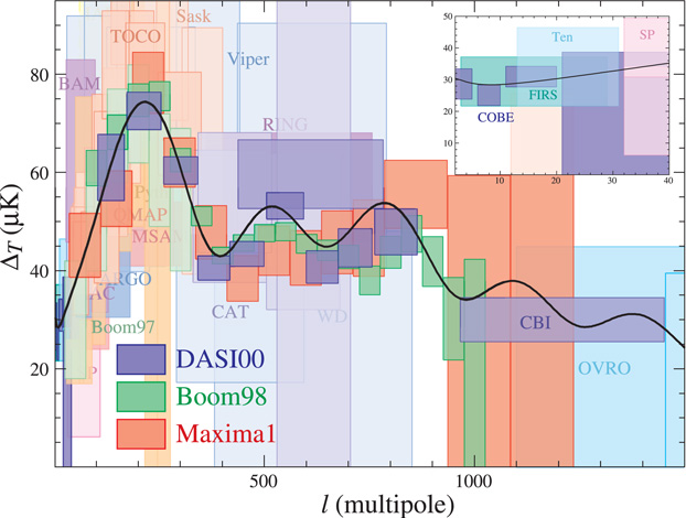
Plate 1 (top) shows observations of
T along
with the prediction of the working cosmological model,
complete with the acoustic peaks mentioned in
Section 1
and discussed extensively in Section 3.
While COBE first detected anisotropy on the
largest scales (inset), observations in the last decade
have pushed the frontier to smaller and smaller scales
(left to right in the figure). The MAP
satellite, launched in June 2001, will go out to
~ 1000, while
the European satellite, Planck, scheduled for launch in 2007, will go
a factor of two higher (see Plate 1 bottom).
 |
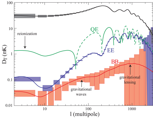 |
Plate 1: Top: temperature anisotropy data
with boxes representing
1- |
The power spectra shown in Plate 1 all begin
at = 2 and
exhibit large errors at low multipoles. The reason is that
the predicted power spectrum is the average power in the multipole moment
an observer would see
in an ensemble of universes. However a real observer is limited to
one Universe and one sky with its one set of
m's,
2 + 1 numbers for each
.
This is particularly problematic for the monopole and dipole
( = 0, 1).
If the monopole were larger in our
vicinity than its average value, we would have no way of knowing it.
Likewise for the dipole, we have no way of distinguishing a cosmological
dipole from our own peculiar motion with respect to the CMB rest frame.
Nonetheless, the monopole and dipole - which we will often call simply
and
v - are of the utmost
significance in the early Universe. It is precisely the
spatial and temporal variation of these quantities, especially
the monopole, which determines the
pattern of anisotropies we observe today. A distant observer sees
spatial variations in the local temperature or monopole, at a distance
given by the lookback time, as a fine-scale angular anisotropy. Similarly,
local dipoles appear as a Doppler shifted temperature
which is viewed analogously. In the jargon of the field,
this simple projection is referred to as the freestreaming of
power from the monopole and dipole to higher multipole moments.
- are of the utmost
significance in the early Universe. It is precisely the
spatial and temporal variation of these quantities, especially
the monopole, which determines the
pattern of anisotropies we observe today. A distant observer sees
spatial variations in the local temperature or monopole, at a distance
given by the lookback time, as a fine-scale angular anisotropy. Similarly,
local dipoles appear as a Doppler shifted temperature
which is viewed analogously. In the jargon of the field,
this simple projection is referred to as the freestreaming of
power from the monopole and dipole to higher multipole moments.
| Name | Authors | Journal Reference |
| ARGO | Masi S et al. 1993 | Ap. J. Lett. 463:L47-L50 |
| ATCA | Subrahmanyan R et al. 2000 | MNRAS 315:808-822 |
| BAM | Tucker GS et al. 1997 | Ap. J. Lett. 475:L73-L76 |
| BIMA | Dawson KS et al. 2001 | Ap. J. Lett. 553:L1-L4 |
| BOOM97 | Mauskopf PD et al. 2000 | Ap. J. Lett. 536:L59-L62 |
| BOOM98 | Netterfield CB et al. 2001 | Ap. J. In press |
| CAT99 | Baker JC et al. 1999 | MNRAS 308:1173-1178 |
| CAT96 | Scott PF et al. 1996 | Ap. J. Lett. 461:L1-L4 |
| CBI | Padin S et al. 2001 | Ap. J. Lett. 549:L1-L5 |
| COBE | Hinshaw G, et al. 1996 | Ap. J. 464:L17-L20 |
| DASI | Halverson NW et al. 2001 | Ap. J. In press |
| FIRS | Ganga K, et al. 1994. | Ap. J. Lett. 432:L15-L18 |
| IAC | Dicker SR et al. 1999 | Ap. J. Lett. 309:750-760 |
| IACB | Femenia B, et al. 1998 | Ap. J. 498:117-136 |
| QMAP | de Oliveira-Costa A et al. 1998 | Ap. J. Lett. 509:L77-L80 |
| MAT | Torbet E et al. 1999 | Ap. J. Lett. 521:L79-L82 |
| MAX | Tanaka ST et al. 1996 | Ap. J. Lett. 468:L81-L84 |
| MAXIMA1 | Lee AT et al. 2001 | Ap. J. In press |
| MSAM | Wilson GW et al. 2000 | Ap. J. 532:57-64 |
| OVRO | Readhead ACS et al. 1989 | Ap. J. 346:566-587 |
| PYTH | Platt SR et al. 1997 | Ap. J. Lett. 475:L1-L4 |
| PYTH5 | Coble K et al. 1999 | Ap. J. Lett. 519:L5-L8 |
| RING | Leitch EM et al. 2000 | Ap. J. 532:37-56 |
| SASK | Netterfield CB et al. 1997 | Ap. J. Lett. 477:47-66 |
| SP94 | Gunderson JO, et al. 1995 | Ap. J. Lett. 443:L57-L60 |
| SP91 | Schuster J et al. 1991 | Ap. J. Lett. 412:L47-L50 |
| SUZIE | Church SE et al. 1997 | Ap. J. 484:523-537 |
| TEN | Gutiérrez CM, et al. 2000 | Ap. J. Lett. 529:47-55 |
| TOCO | Miller AD et al. 1999 | Ap. J. Lett. 524:L1-L4 |
| VIPER | Peterson JB et al. 2000 | Ap. J. Lett. 532:L83-L86 |
| VLA | Partridge RB et al. 1997 | Ap. J. 483:38-50 |
| WD | Tucker GS et al. 1993 | Ap. J. Lett. 419:L45-L49 |
| MAP | http://map.nasa.gsfc.gov | |
| Planck | http://astro.estec.esa.nl/Planck | |
How accurately can the spectra ultimately be measured?
As alluded to above, the fundamental limitation is set by "cosmic
variance" the fact that there are only
2 + 1 m-samples of
the power in each multipole moment. This leads to an inevitable error of
 |
(4) |
Allowing for
further averaging over in
bands of
, we
see that the precision in the power spectrum determination scales as
-1,
i.e. ~ 1% at = 100 and
~ 0.1% at = 1000.
It is the combination of precision predictions and prospects for precision
measurements that gives CMB anisotropies their unique stature.
There are two general caveats to these scalings. The first is that any source of noise, instrumental or astrophysical, increases the errors. If the noise is also Gaussian and has a known power spectrum, one simply replaces the power spectrum on the rhs of Equation (4) with the sum of the signal and noise power spectra [Knox, 1995]. This is the reason that the errors for the Planck satellite increase near its resolution scale in Plate 1 (bottom). Because astrophysical foregrounds are typically non-Gaussian it is usually also necessary to remove heavily contaminated regions, e.g. the galaxy. If the fraction of sky covered is fsky, then the errors increase by a factor of fsky-1/2 and the resulting variance is usually dubbed "sample variance" [Scott et al, 1994]. An fsky = 0.65 was chosen for the Planck satellite.
While no polarization has yet been detected, general considerations of Thomson scattering suggest that up to 10% of the anisotropies at a given scale are polarized. Experimenters are currently hot on the trail, with upper limits approaching the expected level [Hedman et al, 2001, Keating et al, 2001]. Thus, we expect polarization to be an extremely exciting field of study in the coming decade.
The polarization field can be analyzed in a way very similar to the temperature field, save for one complication. In addition to its strength, polarization also has an orientation, depending on relative strength of two linear polarization states. While classical literature has tended to describe polarization locally in terms of the Stokes parameters Q and U 1, recently cosmologists [Seljak, 1997, Kamionkowski et al, 1997, Zaldarriaga & Seljak, 1997] have found that the scalar E and pseudo-scalar B, linear but non-local combinations of Q and U, provide a more useful description. Postponing the precise definition of E and B until Section 3.7, we can, in complete analogy with Equation (1), decompose each of them in terms of multipole moments, and then, following Equation (2), consider the power spectra,
 |
(5) |
Parity invariance demands that the cross correlation between the
pseudoscalar B and the scalars
or E vanishes.
The polarization spectra shown in
Plate 1 [bottom, plotted
in µK following Equation (3)] have several notable
features. First, the amplitude of the EE spectrum is indeed down
from the temperature spectrum by a factor of ten. Second, the
oscillatory structure of the EE spectrum is very similar to the
temperature oscillations, only they are apparently out of phase but
correlated with each other. Both of these features are a direct result
of the simple physics of acoustic oscillations as will be shown in
Section 3. The final feature of the polarization
spectra is the comparative smallness of the BB signal.
Indeed, density perturbations do not produce B modes
to first order. A detection of substantial B polarization,
therefore, would be
momentous. While E polarization effectively doubles our cosmological
information, supplementing that contained in
C,
B detection would push us qualitatively forward into new areas
of physics.
1 There is also the possibility in general of circular polarization, described by Stokes parameter V, but this is absent in cosmological settings. Back.
 errors and approximate