Copyright © 2002 by Annual Reviews. All rights reserved
| Annu. Rev. Astron. Astrophys. 2002. 40:
171-216 Copyright © 2002 by Annual Reviews. All rights reserved |


When the temperature of the Universe was ~ 3000K at a redshift
z*  103, electrons and
protons combined to form neutral hydrogen, an event usually known
as recombination
([Peebles, 1968,
Zel'dovich et al, 1969];
see [Seager et al, 2000] for
recent refinements).
Before this epoch, free electrons acted as glue between the photons
and the baryons through Thomson and Coulomb scattering,
so the cosmological plasma
was a tightly coupled photon-baryon fluid
[Peebles & Yu, 1970].
The spectrum depicted in Plate 1 can be
explained almost completely
by analyzing the behavior of this pre-recombination fluid.
103, electrons and
protons combined to form neutral hydrogen, an event usually known
as recombination
([Peebles, 1968,
Zel'dovich et al, 1969];
see [Seager et al, 2000] for
recent refinements).
Before this epoch, free electrons acted as glue between the photons
and the baryons through Thomson and Coulomb scattering,
so the cosmological plasma
was a tightly coupled photon-baryon fluid
[Peebles & Yu, 1970].
The spectrum depicted in Plate 1 can be
explained almost completely
by analyzing the behavior of this pre-recombination fluid.
In Section 3.1, we start from the two basic equations of fluid mechanics and derive the salient characteristics of the anisotropy spectrum: the existence of peaks and troughs; the spacing between adjacent peaks; and the location of the first peak. These properties depend in decreasing order of importance on the initial conditions, the energy contents of the Universe before recombination and those after recombination. Ironically, the observational milestones have been reached in almost the opposite order. Throughout the 1990's constraints on the location of the first peak steadily improved culminating with precise determinations from the TOCO [Miller et al, 1999], Boomerang, [de Bernardis et al, 2000] and Maxima-1 [Hanany et al, 2000] experiments (see Plate 1 top). In the working cosmological model it shows up right where it should be if the present energy density of the Universe is equal to the critical density, i.e. if the Universe is flat. The skeptic should note that the working cosmological model assumes a particular form for the initial conditions and energy contents of the Universe before recombination which we shall see have only recently been tested directly (with an as yet much lower level of statistical confidence) with the higher peaks.
In Section 3.2 we introduce the initial conditions that apparently are the source of all clumpiness in the Universe. In the context of ab initio models, the term "initial conditions" refers to the physical mechanism that generates the primordial small perturbations. In the working cosmological model, this mechanism is inflation and it sets the initial phase of the oscillations to be the same across all Fourier modes. Remarkably, from this one fact alone comes the prediction that there will be peaks and troughs in the amplitude of the oscillations as a function of wavenumber. Additionally the inflationary prediction of an approximately scale-invariant amplitude of the initial perturbations implies roughly scale-invariant oscillations in the power spectrum. And inflation generically predicts a flat Universe. These are all falsifiable predictions of the simplest inflationary models and they have withstood the test against observations to date.
The energy contents of the Universe before recombination all leave their distinct signatures on the oscillations as discussed in Section 3.3-Section 3.5. In particular, the cold dark matter and baryon signatures have now been seen in the data [Halverson et al, 2001, Netterfield et al, 2001, Lee et al, 2001]. The coupling between electrons and photons is not perfect, especially as one approaches the epoch of recombination. As discussed in Section 3.6, this imperfect coupling leads to damping in the anisotropy spectrum: very small scale inhomogeneities are smoothed out. The damping phenomenon has now been observed by the CBI experiment [Padin et al, 2001]. Importantly, fluid imperfections also generate linear polarization as covered in Section 3.7. Because the imperfection is minimal and appears only at small scales, the polarization generated is small and has not been detected to date.
After recombination the photons basically travel freely to us today, so the problem of translating the acoustic inhomogeneities in the photon distribution at recombination to the anisotropy spectrum today is simply one of projection. This projection depends almost completely on one number, the angular diameter distance between us and the surface of last scattering. That number depends on the energy contents of the Universe after recombination through the expansion rate. The hand waving projection argument of Section 3.1 is formalized in Section 3.8, in the process introducing the popular code used to compute anisotropies, CMBFAST. Finally, we discuss the sensitivity of the acoustic peaks to cosmological parameters in Section 3.9.
For pedagogical purposes, let us begin with an idealization of a perfect photon-baryon fluid and neglect the dynamical effects of gravity and the baryons. Perturbations in this perfect fluid can be described by a simple continuity and an Euler equation that encapsulate the basic properties of acoustic oscillations.
The discussion of acoustic oscillations will take place exclusively in Fourier space. For example, we decompose the monopole of the temperature field into
 |
(6) |
and omit the subscript 00 on the Fourier amplitude.
Since perturbations
are very small, the evolution equations are linear, and different Fourier
modes evolve independently. Therefore, instead of partial differential
equations for a field
 (x), we have
ordinary differential equations for
(k). In fact,
due to rotational symmetry, all
(k) for a
given k obey the same equations. Here and in the following sections,
we omit the wavenumber argument k where no
confusion with physical space quantities will arise.
(x), we have
ordinary differential equations for
(k). In fact,
due to rotational symmetry, all
(k) for a
given k obey the same equations. Here and in the following sections,
we omit the wavenumber argument k where no
confusion with physical space quantities will arise.
Temperature perturbations in Fourier space obey
 |
(7) |
This equation for the photon temperature
, which does indeed
look like the familiar continuity equation
in Fourier space (derivatives
 become wavenumbers
k), has
a number of subtleties hidden in it, due to the cosmological setting.
First, the "time" derivative here is actually with respect to
conformal time
become wavenumbers
k), has
a number of subtleties hidden in it, due to the cosmological setting.
First, the "time" derivative here is actually with respect to
conformal time


 dt
/ a(t).
Since we are working in units in which the speed of light c = 1,
is also the
maximum comoving distance a particle could have traveled
since t = 0. It is often called
the comoving horizon or more specifically the comoving
particle horizon. The physical horizon is a times the
comoving horizon.
dt
/ a(t).
Since we are working in units in which the speed of light c = 1,
is also the
maximum comoving distance a particle could have traveled
since t = 0. It is often called
the comoving horizon or more specifically the comoving
particle horizon. The physical horizon is a times the
comoving horizon.
Second, the photon fluid velocity here
v has been written as a scalar instead of a vector.
In the early universe, only the velocity component parallel to the
wavevector k is
expected to be important, since they alone have a source in gravity.
Specifically,
v = - iv
has been written as a scalar instead of a vector.
In the early universe, only the velocity component parallel to the
wavevector k is
expected to be important, since they alone have a source in gravity.
Specifically,
v = - iv
 .
In terms of the moments introduced in Section 2,
v
represents a dipole moment directed along k.
The factor of 1/3 comes about since continuity conserves photon number
not temperature and the number density
n
.
In terms of the moments introduced in Section 2,
v
represents a dipole moment directed along k.
The factor of 1/3 comes about since continuity conserves photon number
not temperature and the number density
n
 T3.
Finally, we emphasize that, for the time being, we are neglecting the
effects of gravity.
T3.
Finally, we emphasize that, for the time being, we are neglecting the
effects of gravity.
The Euler equation for a fluid is an expression of momentum conservation.
The momentum density of the photons is
( +
p)
v, where the photon pressure
p =
/ 3.
In the absence of gravity and viscous fluid imperfections, pressure
gradients
p =
/ 3
supply the only force. Since
T4,
this becomes
4k
+
p)
v, where the photon pressure
p =
/ 3.
In the absence of gravity and viscous fluid imperfections, pressure
gradients
p =
/ 3
supply the only force. Since
T4,
this becomes
4k
 / 3 in Fourier space. The Euler equation then becomes
 |
(8) |
Differentiating the continuity equation and inserting the Euler equation yields the most basic form of the oscillator equation
 |
(9) |
where cs
( /
/
 )1/2 = 1 / 31/2 is the sound speed
in the (dynamically baryon-free) fluid.
What this equation says is that pressure gradients act as a
restoring force to any initial perturbation in the system which thereafter
oscillate at the speed of sound. Physically these temperature
oscillations represent the heating and cooling of a fluid that
is compressed and rarefied by a standing sound or acoustic wave.
This behavior continues until recombination. Assuming negligible
initial velocity perturbations, we have a temperature distribution at
recombination of
)1/2 = 1 / 31/2 is the sound speed
in the (dynamically baryon-free) fluid.
What this equation says is that pressure gradients act as a
restoring force to any initial perturbation in the system which thereafter
oscillate at the speed of sound. Physically these temperature
oscillations represent the heating and cooling of a fluid that
is compressed and rarefied by a standing sound or acoustic wave.
This behavior continues until recombination. Assuming negligible
initial velocity perturbations, we have a temperature distribution at
recombination of
 |
(10) |
where
s =
cs
d
/
31/2 is the distance sound can
travel by ,
usually called the sound horizon. Asterisks denote
evaluation at recombination z*.
In the limit of scales large compared with the sound horizon ks
<< 1,
the perturbation is frozen into its initial conditions. This is the gist of
the statement that the large-scale anisotropies measured by COBE directly
measure the initial conditions. On small scales, the amplitude of the
Fourier modes will exhibit temporal oscillations, as shown in
Figure 1
[with  = 0,
i =
3(0) for this
idealization].
Modes that are caught at maxima or minima of their oscillation at
recombination correspond to peaks in the
power, i.e. the variance of
(k,
*). Because
sound takes half as long to travel half as far, modes corresponding
to peaks follow a harmonic relationship
kn = n
= 0,
i =
3(0) for this
idealization].
Modes that are caught at maxima or minima of their oscillation at
recombination correspond to peaks in the
power, i.e. the variance of
(k,
*). Because
sound takes half as long to travel half as far, modes corresponding
to peaks follow a harmonic relationship
kn = n
 /
s*, where n is an integer (see
Figure 1a).
/
s*, where n is an integer (see
Figure 1a).
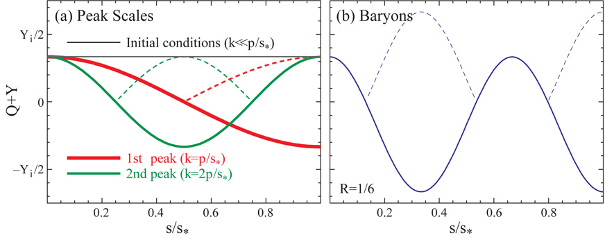 |
Figure 1. Idealized acoustic oscillations. (a) Peak scales: the wavemode that completes half an oscillation by recombination sets the physical scale of the first peak. Both minima and maxima correspond to peaks in power (dashed lines, absolute value) and so higher peaks are integral multiples of this scale with equal height. Plotted here is the idealization of Equation (15) (constant potentials, no baryon loading). (b) Baryon loading. Baryon loading boosts the amplitudes of every other oscillation. Plotted here is the idealization of Equation (16) (constant potentials and baryon loading R = 1/6) for the third peak. |
How does this spectrum of inhomogeneities at recombination
appear to us today? Roughly speaking, a spatial inhomogeneity
in the CMB temperature of wavelength
 appears as an angular
anisotropy of scale
appears as an angular
anisotropy of scale
 / D where
D(z) is the
comoving angular diameter distance from the observer to redshift
z. We will address this issue more formally in
Section 3.8. In a flat universe,
D* =
0 -
*
0, where
0
(z = 0).
In harmonic space, the relationship implies a coherent series of
acoustic peaks in the anisotropy spectrum, located at
/ D where
D(z) is the
comoving angular diameter distance from the observer to redshift
z. We will address this issue more formally in
Section 3.8. In a flat universe,
D* =
0 -
*
0, where
0
(z = 0).
In harmonic space, the relationship implies a coherent series of
acoustic peaks in the anisotropy spectrum, located at
 |
(11) |
To get a feel for where these features should appear, note that in a
flat matter dominated universe
(1 +
z)-1/2 so that * /
0
1/30
2°. Equivalently
 1
200. Notice that
since we are measuring ratios of distances
the absolute distance scale drops out; we shall see in
Section 3.5
that the Hubble constant sneaks back into the problem because the Universe
is not fully matter-dominated at recombination.
1
200. Notice that
since we are measuring ratios of distances
the absolute distance scale drops out; we shall see in
Section 3.5
that the Hubble constant sneaks back into the problem because the Universe
is not fully matter-dominated at recombination.
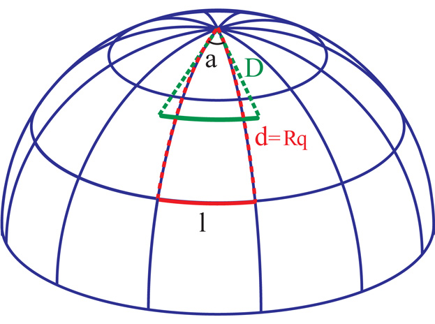 |
Figure 2. Angular diameter distance. In a
closed universe, objects are
further than they appear to be from Euclidean (flat) expectations
corresponding to the difference between coordinate distance d and
angular diameter distance D. Consequently, at a fixed coordinate
distance, a given angle corresponds to a smaller spatial scale in
a closed universe. Acoustic peaks therefore appear at larger
angles or lower |
In a spatially curved universe, the angular diameter distance
no longer equals the coordinate distance making the peak locations
sensitive to the spatial curvature of the Universe
[Doroshkevich et al, 1978,
Kamionkowski et al, 1994].
Consider first a closed universe with radius of curvature
R = H0-1
| tot -
1|-1/2. Suppressing one spatial coordinate yields
a 2-sphere geometry with the observer situated at the
pole (see Figure 2). Light travels on
lines of longitude.
A physical scale at
fixed latitude given by
the polar angle
subtends an angle
tot -
1|-1/2. Suppressing one spatial coordinate yields
a 2-sphere geometry with the observer situated at the
pole (see Figure 2). Light travels on
lines of longitude.
A physical scale at
fixed latitude given by
the polar angle
subtends an angle  =
/ R
sin .
For << 1,
a Euclidean analysis would infer a distance
D = R sin ,
even though the coordinate distance along the arc is
d = R; thus
=
/ R
sin .
For << 1,
a Euclidean analysis would infer a distance
D = R sin ,
even though the coordinate distance along the arc is
d = R; thus
 |
(12) |
For open universes, simply replace sin with sinh.
The result is that objects in an open (closed) universe are closer
(further) than they appear, as if seen through a lens.
In fact one way of viewing this effect is as the gravitational
lensing due to the background density (c.f.
Section 4.2.4).
A given comoving scale at a fixed distance subtends
a larger (smaller) angle in a closed (open) universe than a flat universe.
This strong scaling with spatial curvature indicates that
the observed first peak at
1
200 constrains
the geometry to be nearly spatially flat. We will implicitly
assume spatial flatness in the following sections unless otherwise
stated.
Finally in a flat dark energy dominated universe, the conformal age of
the Universe decreases approximately as
0
 0(1
+ lnm0.085). For reasonable
m, this
causes only a small shift
of 1 to lower
multipoles (see Plate 4) relative
to the effect of curvature. Combined with the effect of
the radiation near recombination, the peak locations provides a means to
measure the physical age t0 of a flat universe
[Hu et al, 2001].
0(1
+ lnm0.085). For reasonable
m, this
causes only a small shift
of 1 to lower
multipoles (see Plate 4) relative
to the effect of curvature. Combined with the effect of
the radiation near recombination, the peak locations provides a means to
measure the physical age t0 of a flat universe
[Hu et al, 2001].
As suggested above, observations of the location of the first peak strongly
point to a flat universe. This is encouraging news for adherents of
inflation, a theory which initially predicted
tot = 1
at a time when few astronomers would sign on to such a high value (see
[Liddle & Lyth, 1993]
for a review).
However, the argument
for inflation goes beyond the confirmation of flatness. In particular,
the discussion of the last subsection begs the question: whence
(0),
the initial conditions of the temperature fluctuations? The answer requires
the inclusion of gravity and considerations of causality which point
to inflation as the origin of structure in the Universe.
The calculations of the typical angular scale of the acoustic oscillations in the last section are familiar in another context: the horizon problem. Because the sound speed is near the speed of light, the degree scale also marks the extent of a causally connected region or particle horizon at recombination. For the picture in the last section to hold, the perturbations must have been laid down while the scales in question were still far outside the particle horizon 2. The recent observational verification of this basic peak structure presents a problem potentially more serious than the original horizon problem of approximate isotropy: the mechanism which smooths fluctuations in the Universe must also regenerate them with superhorizon sized correlations at the 10-5 level. Inflation is an idea that solves both problems simultaneously.
The inflationary paradigm postulates that an early phase of near exponential expansion of the Universe was driven by a form of energy with negative pressure. In most models, this energy is usually provided by the potential energy of a scalar field. The inflationary era brings the observable universe to a nearly smooth and spatially flat state. Nonetheless, quantum fluctuations in the scalar field are unavoidable and also carried to large physical scales by the expansion. Because an exponential expansion is self-similar in time, the fluctuations are scale-invariant, i.e. in each logarithmic interval in scale the contribution to the variance of the fluctuations is equal. Since the scalar field carries the energy density of the Universe during inflation, its fluctuations induce variations in the spatial curvature [Guth & Pi, 1985, Hawking, 1982, Bardeen et al, 1983]. Instead of perfect flatness, inflation predicts that each scale will resemble a very slightly open or closed universe. This fluctuation in the geometry of the Universe is essentially frozen in while the perturbation is outside the horizon [Bardeen, 1980].
Formally, curvature fluctuations are perturbations to the space-space
piece of the metric. In a Newtonian coordinate system, or gauge, where
the metric is diagonal, the spatial curvature fluctuation is called
 gij =
2a2
gij =
2a2
 ij (see e.g.
[Ma & Bertschinger, 1995]).
The more familiar Newtonian potential is the time-time fluctuation
gtt =
2 and is
approximately
-
. Approximate scale
invariance then says that
ij (see e.g.
[Ma & Bertschinger, 1995]).
The more familiar Newtonian potential is the time-time fluctuation
gtt =
2 and is
approximately
-
. Approximate scale
invariance then says that
 2
k3
P(k) /
22
kn-1
where P(k) is the
power spectrum of and
the tilt n 1.
2
k3
P(k) /
22
kn-1
where P(k) is the
power spectrum of and
the tilt n 1.
Now let us relate the inflationary prediction of scale-invariant
curvature fluctuations to the initial temperature fluctuations.
Newtonian intuition based on the Poisson equation
k2 =
4 Ga2
tells us that on
large scales (small k) density and hence temperature
fluctuations should be negligible compared with Newtonian potential.
General relativity says otherwise because the Newtonian potential is also
a time-time fluctuation in the metric. It corresponds to a temporal shift of
t / t =
. The CMB temperature
varies as the inverse of the
scale factor, which in turn depends on time as
a
t2/[3(1+p/)]. Therefore, the fractional change in the
CMB temperature
 |
(13) |
Thus, a temporal shift produces a temperature perturbation of
- / 2 in the radiation
dominated era (when p =
/ 3) and
-2 / 3 in the matter
dominated epoch (p = 0)
([Peacock, 1991];
[White & Hu, 1997]).
The initial temperature perturbation is
therefore inextricably linked with the initial gravitational potential
perturbation. Inflation predicts scale-invariant initial
fluctuations in both the CMB temperature and the spatial curvature
in the Newtonian gauge.
Alternate models which seek to obey the causality can generate curvature
fluctuations only inside the particle horizon. Because the perturbations
are then not generated at the same epoch independent of scale, there is
no longer a unique
relationship between the phase of the oscillators. That is, the argument
of the cosine in Equation (10) becomes ks* +
 (k),
where is a phase
which can in principle be different for different wavevectors,
even those with the same magnitude k. This can lead to
temporal incoherence in the oscillations and
hence a washing out of the acoustic peaks
[Albrecht et al, 1996],
most notably in cosmological defect models
[Allen et al, 1997,
Seljak et al, 1997].
Complete incoherence is not a strict requirement of causality since there
are other ways to synch up the oscillations. For example, many
isocurvature models, where the initial spatial curvature is unperturbed,
are coherent since their oscillations
begin with the generation of curvature fluctuations at horizon
crossing
[Hu & White, 1996].
Still they typically have
(k),
where is a phase
which can in principle be different for different wavevectors,
even those with the same magnitude k. This can lead to
temporal incoherence in the oscillations and
hence a washing out of the acoustic peaks
[Albrecht et al, 1996],
most notably in cosmological defect models
[Allen et al, 1997,
Seljak et al, 1997].
Complete incoherence is not a strict requirement of causality since there
are other ways to synch up the oscillations. For example, many
isocurvature models, where the initial spatial curvature is unperturbed,
are coherent since their oscillations
begin with the generation of curvature fluctuations at horizon
crossing
[Hu & White, 1996].
Still they typically have
 0 (c.f.
[Turok, 1996]).
Independent of the angular diameter distance
D*, the ratio of the peak locations gives the
phase: 1 :
2 :
3 ~ 1 : 2 :
3 for = 0.
Likewise independent of a constant phase, the spacing of the peaks
n -
n-1 =
A gives a measure
of the angular diameter distance
[Hu & White, 1996].
The observations, which indicate coherent oscillations with
= 0,
therefore have provided a non-trivial test of
the inflationary paradigm and supplied
a substantially more stringent version of the horizon problem
for contenders to solve.
0 (c.f.
[Turok, 1996]).
Independent of the angular diameter distance
D*, the ratio of the peak locations gives the
phase: 1 :
2 :
3 ~ 1 : 2 :
3 for = 0.
Likewise independent of a constant phase, the spacing of the peaks
n -
n-1 =
A gives a measure
of the angular diameter distance
[Hu & White, 1996].
The observations, which indicate coherent oscillations with
= 0,
therefore have provided a non-trivial test of
the inflationary paradigm and supplied
a substantially more stringent version of the horizon problem
for contenders to solve.
We saw above that fluctuations in a scalar field during inflation
get turned into temperature fluctuations via the intermediary of gravity.
Gravity affects in
more ways than this. The Newtonian potential and spatial curvature alter
the acoustic oscillations by providing a gravitational force on
the oscillator. The Euler equation (8)
gains a term on the rhs due to the gradient of
the potential k.
The main effect of gravity then is
to make the oscillations a competition between pressure
gradients k
and potential gradients
k with
an equilibrium when +
= 0.
Gravity also changes the continuity equation. Since the Newtonian
curvature is essentially a perturbation to the scale factor, changes
in its value also generate temperature perturbations by analogy to
the cosmological redshift
= -
and so
the continuity equation (7) gains a contribution of -
 on
the rhs.
on
the rhs.
These two effects bring the oscillator equation (9) to
 |
(14) |
In a flat universe and in the absence
of pressure, and
are constant. Also, in
the absence of baryons,
cs2 = 1/3 so the new oscillator equation
is identical to Equation (9) with
replaced by
+
. The solution
in the matter dominated epoch is then
 |
(15) |
where
md
represents the start of the matter dominated epoch
(see Figure 1a).
We have used the matter dominated "initial conditions" for
given in the previous section assuming large scales,
ksmd << 1.
The results from the idealization of
Section 3.1 carry through with a few exceptions. Even
without an initial temperature fluctuation to displace the oscillator,
acoustic oscillations would arise by the infall and compression
of the fluid into gravitational
potential wells. Since it is the effective temperature
+
that oscillates, they
occur even if
(0) = 0. The quantity
+
can be thought of as an
effective temperature in another way: after recombination, photons
must climb out of the potential well to the observer and thus suffer
a gravitational redshift of
T / T
= . The effective
temperature fluctuation is therefore also the observed temperature
fluctuation. We now see that the large scale limit of
Equation (15) recovers the famous Sachs-Wolfe result
that the observed temperature perturbation is
/ 3
and overdense regions correspond to cold spots on the sky
[Sachs & Wolfe, 1967].
When < 0, although
is positive, the
effective temperature
+
is negative.
The plasma begins effectively rarefied in gravitational potential wells.
As gravity compresses the fluid and pressure resists, rarefaction becomes
compression and rarefaction again. The first peak corresponds to the
mode that is caught in its first compression
by recombination. The second peak at roughly half the wavelength corresponds
to the mode that went through a full cycle of compression and rarefaction
by recombination. We will use this language of the compression
and rarefaction phase inside initially overdense regions but one should bear
in mind that there are an equal number of initially underdense regions
with the opposite phase.
So far we have been neglecting the baryons in the dynamics of
the acoustic oscillations. To see whether this is a reasonable
approximation consider the photon-baryon momentum density
ratio R = (pb +
b
/ (p
+ )
30b
h2(z / 103)-1. For
typical values of
the baryon density this number is of order unity at recombination
and so we expect baryonic effects to begin appearing in the oscillations
just as they are frozen in.
Baryons are conceptually easy to include in the evolution equations since their momentum density provides extra inertia in the joint Euler equation for pressure and potential gradients to overcome. Since inertial and gravitational mass are equal, all terms in the Euler equation save the pressure gradient are multiplied by 1 + R leading to the revised oscillator equation [Hu & Sugiyama, 1995]
 |
(16) |
where we have used the fact that the sound speed is reduced by the baryons to cs = 1 / [3(1 + R)]1/2.
To get a feel for the implications of the baryons take the limit
of constant R,
and . Then
d2(R
) /
d2(= 0) may be added to the left hand side to
again put the oscillator equation
in the form of Equation (9) with
+ (1 +
R).
The solution then becomes
 |
(17) |
Aside from the lowering of the sound speed which decreases the sound
horizon, baryons have two distinguishing effects:
they enhance the amplitude of the oscillations and shift the equilibrium
point to
= - (1 +
R) (see
Figure 1b).
These two effects are intimately related
and are easy to understand since the equations are exactly those of
a mass m = 1 + R
on a spring in a constant gravitational field.
For the same initial conditions, increasing the mass causes the oscillator
to fall further in the gravitational field leading to larger oscillations
and a shifted zero point.
The shifting of the zero point of the oscillator has significant
phenomenological consequences. Since it is still the effective temperature
+
that is the observed
temperature, the zero point shift
breaks the symmetry of the oscillations. The baryons
enhance only the compressional phase, i.e. every other peak. For
the working cosmological model these are the first, third, fifth...
Physically, the extra gravity provided by the baryons enhance
compression into potential wells.
These qualitative results
remain true in the presence of a time-variable R. An additional
effect arises due to the adiabatic damping of an oscillator with
a time-variable mass. Since the energy/frequency of an oscillator
is an adiabatic invariant, the amplitude must decay as
(1 + R)-1/4.
This can also be understood by expanding the time derivatives in
Equation (16) and identifying the

 term
as the remnant of the familiar expansion drag on baryon velocities.
term
as the remnant of the familiar expansion drag on baryon velocities.
We have hitherto also been neglecting the energy density of the radiation in
comparison to the matter. The matter-to-radiation ratio scales as
m
/ r
24m
h2(z / 103)-1
and so is also of order unity at recombination for reasonable parameters.
Moreover fluctuations corresponding to the higher peaks entered the
sound horizon at an earlier time, during radiation domination.
Including the radiation changes the expansion rate of the Universe and hence the physical scale of the sound horizon at recombination. It introduces yet another potential ambiguity in the interpretation of the location of the peaks. Fortunately, the matter-radiation ratio has another effect in the power spectrum by which it can be distinguished. Radiation drives the acoustic oscillations by making the gravitational force evolve with time [Hu & Sugiyama, 1995]. Matter does not.
The exact evolution of the potentials is determined by the relativistic Poisson equation. But qualitatively, we know that the background density is decreasing with time, so unless the density fluctuations in the dominant component grow unimpeded by pressure, potentials will decay. In particular, in the radiation dominated era once pressure begins to fight gravity at the first compressional maxima of the wave, the Newtonian gravitational potential and spatial curvature must decay (see Figure 3).
 |
Figure 3. Radiation driving and diffusion
damping. The decay of the potential
|
This decay actually drives the
oscillations: it is timed to leave the fluid maximally compressed with
no gravitational potential to fight as it turns around.
The net effect is doubled since the redshifting from the spatial metric
fluctuation also goes
away at the same time. When the Universe becomes matter dominated
the gravitational potential is no longer determined by
photon-baryon density perturbations but by the pressureless
cold dark matter. Therefore, the amplitudes of the acoustic peaks
increase as the cold dark matter-to-radiation ratio decreases
[Seljak, 1994,
Hu & Sugiyama, 1995].
Density perturbations in any form of radiation will stop growing around
horizon crossing and lead to this effect. The net result is that across
the horizon scale at matter radiation equality
(keq
(4 - 2 2) /
eq)
the acoustic amplitude increases by a factor of 4-5
[Hu & Sugiyama, 1996].
By eliminating gravitational potentials, photon-baryon acoustic
oscillations eliminate the alternating peak heights from baryon loading.
The observed high third peak
[Halverson et al, 2001]
is a good indication that cold dark matter both exists and dominates the
energy density at recombination.
2) /
eq)
the acoustic amplitude increases by a factor of 4-5
[Hu & Sugiyama, 1996].
By eliminating gravitational potentials, photon-baryon acoustic
oscillations eliminate the alternating peak heights from baryon loading.
The observed high third peak
[Halverson et al, 2001]
is a good indication that cold dark matter both exists and dominates the
energy density at recombination.
The photon-baryon fluid has slight imperfections corresponding to shear viscosity and heat conduction in the fluid [Weinberg, 1971]. These imperfections damp acoustic oscillations. To consider these effects, we now present the equations of motion of the system in their full form, including separate continuity and Euler equations for the baryons. Formally the continuity and Euler equations follow from the covariant conservation of the joint stress-energy tensor of the photon-baryon fluid. Because photon and baryon numbers are separately conserved, the continuity equations are unchanged,
 |
(18) |
where b and
vb are the density perturbation and
fluid velocity of the baryons.
The Euler equations contain qualitatively new terms
 |
(19) |
For the baryons
the first term on the right accounts for cosmological expansion,
which makes momenta decay as a-1. The third term on
the right accounts for momentum exchange in the Thomson scattering
between photons and electrons (protons are very tightly coupled to
electrons via Coulomb scattering), with
 ne
ne
 T a
the differential Thomson
optical depth, and is compensated by its opposite in the photon Euler
equation. These terms are the origin of heat conduction imperfections.
If the medium is optically thick across a wavelength,
/ k >> 1
and the photons and baryons cannot slip past each other.
As it becomes optically thin, slippage dissipates the fluctuations.
T a
the differential Thomson
optical depth, and is compensated by its opposite in the photon Euler
equation. These terms are the origin of heat conduction imperfections.
If the medium is optically thick across a wavelength,
/ k >> 1
and the photons and baryons cannot slip past each other.
As it becomes optically thin, slippage dissipates the fluctuations.
In the photon Euler equation there is an extra force on the rhs
due to anisotropic stress gradients or radiation viscosity in the
fluid, . The
anisotropic stress is directly proportional to the
quadrupole moment of the photon temperature distribution.
A quadrupole moment is established by gradients in
v
as photons from say neighboring temperature crests meet at
a trough (see Plate 3, inset).
However it is destroyed by scattering. Thus
=
2(kv /
)
Av, where the order
unity constant can be derived from the Boltzmann equation
Av = 16/15
[Kaiser, 1983].
Its evolution is shown in
Figure 3. With
the continuity Equation (7),
kv
-3 and
so viscosity takes the form of a damping term.
The heat conduction term can be shown to have a similar effect
by expanding the Euler equations in
k / .
The final oscillator equation including both terms becomes
 |
(20) |
where the heat conduction coefficient
Ah = R2 / (1 + R).
Thus we expect the
inhomogeneities to be damped by a exponential factor of order
e-k2 /
(see
Figure 3).
The damping scale kd is thus of order
( /
)1/2,
corresponding to the geometric mean of the horizon and the mean free path.
Damping can be thought of
as the result of the random walk in the baryons that takes photons
from hot regions into cold and vice-versa
[Silk, 1968].
Detailed numerical integration of the equations
of motion are required to track the rapid growth of the mean free path
and damping length through recombination itself.
These calculations show that the damping scale is of order
kds*
10
leading to a substantial suppression of the oscillations beyond the
third peak.
How does this suppression depend on the cosmological parameters? As the
matter density
m
h2 increases, the horizon
* decreases
since the expansion rate goes up.
Since the diffusion length is proportional to
(*)1/2, it too decreases
as the matter density goes up but not as much as the angular diameter
distance D* which is also inversely
proportional to the expansion rate.
Thus, more matter translates into more damping at a fixed multipole moment;
conversely, it corresponds to slightly less damping at a fixed peak number.
The dependence on baryons is controlled by the mean free path which
is in turn controlled by the free electron density:
the increase in electron density due to an increase in the
baryons is partially offset by a decrease in the ionization fraction due
to recombination. The net result under the Saha approximation is that the
damping length scales approximately as
(b
h2)-1/4.
Accurate fitting formulae for this scale in terms of
cosmological parameters can be found in
[Hu & White, 1997c].
The dissipation of the acoustic oscillations leaves a signature in
the polarization of CMB in its wake (see e.g.
[Hu & White, 1997a] and
references therein for a more complete treatment).
Much like reflection off of a surface, Thomson scattering induces
a linear polarization in the scattered radiation.
Consider incoming radiation in the - x direction scattered at right
angles into the z direction (see Plate 2,
left panel).
Heuristically, incoming radiation shakes an electron in the direction
of its electric field vector or polarization
 causing it to radiate with an outgoing polarization parallel to that
direction. However since the outgoing polarization
causing it to radiate with an outgoing polarization parallel to that
direction. However since the outgoing polarization
 must be orthogonal to the outgoing direction, incoming radiation that
is polarized parallel to the outgoing direction cannot scatter leaving
only one polarization state.
More generally, the Thomson differential
cross section
dT
/ d
|
.
|2.
must be orthogonal to the outgoing direction, incoming radiation that
is polarized parallel to the outgoing direction cannot scatter leaving
only one polarization state.
More generally, the Thomson differential
cross section
dT
/ d
|
.
|2.
Unlike the reflection of sunlight off of a surface, the incoming
radiation comes from all angles. If it were completely isotropic in
intensity, radiation coming along the
 would
provide the polarization state that is missing from that coming along
would
provide the polarization state that is missing from that coming along
 leaving the net outgoing radiation unpolarized.
Only a quadrupole temperature anisotropy in the radiation
generates a net linear polarization from Thomson scattering.
As we have seen, a quadrupole
can only be generated causally by the motion of photons and then only
if the Universe is optically thin to Thomson
scattering across this scale (i.e. it is inversely proportional to
).
Polarization generation suffers
from a Catch-22: the scattering which generates polarization also
suppresses its quadrupole source.
leaving the net outgoing radiation unpolarized.
Only a quadrupole temperature anisotropy in the radiation
generates a net linear polarization from Thomson scattering.
As we have seen, a quadrupole
can only be generated causally by the motion of photons and then only
if the Universe is optically thin to Thomson
scattering across this scale (i.e. it is inversely proportional to
).
Polarization generation suffers
from a Catch-22: the scattering which generates polarization also
suppresses its quadrupole source.
The fact that the polarization strength is of order the quadrupole
explains the shape and height of the polarization spectra in
Plate 1b.
The monopole and dipole
and
v are of the same order of magnitude
at recombination, but their oscillations are
/ 2 out of phase as follows from
Equation (9) and Equation (10). Since the quadrupole is of order
kv /
(see Figure 3), the polarization
spectrum should be smaller than the temperature spectrum by a factor of
order k /
at recombination. As in the case of the damping, the precise value requires
numerical work
[Bond & Efstathiou, 1987]
since changes so
rapidly near recombination. Calculations show
a steady rise in the polarized fraction with increasing l or
k to a maximum of about ten percent before damping destroys the
oscillations and hence the dipole source. Since
v is out of
phase with the monopole, the polarization peaks should also be out of
phase with the temperature peaks. Indeed,
Plate 1b shows that this is the case.
Furthermore, the phase relation also tells us that the polarization is
correlated with the temperature perturbations. The correlation power
CE
being the product of the two, exhibits oscillations at twice the
acoustic frequency.
Until now, we have focused on the polarization strength without regard to its orientation. The orientation, like a 2 dimensional vector, is described by two components E and B. The E and B decomposition is simplest to visualize in the small scale limit, where spherical harmonic analysis coincides with Fourier analysis [Seljak, 1997]. Then the wavevector k picks out a preferred direction against which the polarization direction is measured (see Plate 2, right panel). Since the linear polarization is a "headless vector" that remains unchanged upon a 180° rotation, the two numbers E and B that define it represent polarization aligned or orthogonal with the wavevector (positive and negative E) and crossed at ± 45° (positive and negative B).
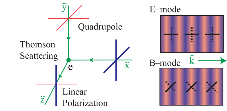 |
Plate 2. Polarization generation and
classification. Left: Thomson scattering of quadrupole temperature
anisotropies (depicted here in the
|
In linear theory, scalar perturbations like the gravitational potential and temperature perturbations have only one intrinsic direction associated with them, that provided by k, and the orientation of the polarization inevitably takes it cue from that one direction, thereby producing an E -mode. The generalization to an all-sky characterization of the polarization changes none of these qualitative features. The E -mode and the B -mode are formally distinguished by the orientation of the Hessian of the Stokes parameters which define the direction of the polarization itself. This geometric distinction is preserved under summation of all Fourier modes as well as the generalization of Fourier analysis to spherical harmonic analysis.
The acoustic peaks in the polarization appear exclusively in the EE power spectrum of Equation (5). This distinction is very useful as it allows a clean separation of this effect from those occuring beyond the scope of the linear perturbation theory of scalar fluctuations: in particular, gravitational waves (see Section 4.2.3) and gravitational lensing (see Section 4.2.4). Moreover, in the working cosmological model, the polarization peaks and correlation are precise predictions of the temperature peaks as they depend on the same physics. As such their detection would represent a sharp test on the implicit assumptions of the working model, especially its initial conditions and ionization history.
The discussion in the previous sections suffices for a qualitative understanding of the acoustic peaks in the power spectra of the temperature and polarization anisotropies. To refine this treatment we must consider more carefully the sources of anisotropies and their projection into multipole moments.
Because the description of the acoustic oscillations takes place
in Fourier space, the projection of inhomogeneities at recombination
onto anisotropies today has an added level of complexity.
An observer today sees the acoustic oscillations
in effective temperature as they appeared on a spherical shell at
x = D*
 at recombination, where
is the direction vector,
and D* =
0 -
* is
the distance light can travel between recombination and the present
(see Plate 3).
Having solved for the Fourier amplitude
[ +
](k,
*), we can expand the
exponential in Equation (6) in terms of spherical harmonics, so the
observed anisotropy today is
at recombination, where
is the direction vector,
and D* =
0 -
* is
the distance light can travel between recombination and the present
(see Plate 3).
Having solved for the Fourier amplitude
[ +
](k,
*), we can expand the
exponential in Equation (6) in terms of spherical harmonics, so the
observed anisotropy today is
 |
(21) |
where the projected source
a(k) =
[ +
](k,
*)
j(kD*).
Because the spherical harmonics are orthogonal, Equation (1) implies that
m today is given by the
integral in square brackets today.
A given plane wave actually produces a range of anisotropies in
angular scale as is obvious from Plate 3. The
one-to-one mapping between wavenumber and multipole moment described in
Section 3.1
is only approximately true and comes from the fact that the
spherical Bessel function
j(kD*) is strongly peaked
at kD*
. Notice that this peak
corresponds to contributions in the direction orthogonal to the
wavevector where the correspondence
between and k is
one-to-one (see Plate 3).
 |
Plate 3. Integral approach. CMB anisotropies can be thought of as the line-of-sight projection of various sources of plane wave temperature and polarization fluctuations: the acoustic effective temperature and velocity or Doppler effect (see Section 3.8), the quadrupole sources of polarization (see Section 3.7) and secondary sources (see Section 4.2, Section 4.3). Secondary contributions differ in that the region over which they contribute is thick compared with the last scattering surface at recombination and the typical wavelength of a perturbation. |
Projection is less straightforward for other sources of anisotropy.
We have hitherto neglected the fact that the acoustic motion of
the photon-baryon fluid also produces a Doppler shift in the radiation
that appears to the observer as a temperature anisotropy as well.
In fact, we argued above that
vb
v is
of comparable magnitude but out of phase with the effective temperature.
If the Doppler effect projected in the same way as the effective
temperature,
it would wash out the acoustic peaks. However, the Doppler effect has
a directional dependence as well since it is only the line-of-sight
velocity that produces the effect. Formally, it is a dipole source
of temperature anisotropies and hence has an
= 1 structure.
The coupling of the dipole and plane wave angular momenta
imply that in the projection of the Doppler effect involves a
combination of j±1 that may be rewritten as
j'(x)
dj(x) / dx.
The structure of j' lacks a strong peak
at x = .
Physically this corresponds to the fact that the
velocity is irrotational and hence has no component in the direction
orthogonal to the wavevector (see Plate 3).
Correspondingly, the Doppler effect cannot produce strong peak structures
[Hu & Sugiyama, 1995].
The observed peaks must be acoustic peaks in the
effective temperature not "Doppler peaks".
There is one more subtlety involved when passing from acoustic oscillations
to anisotropies. Recall from
Section 3.5 that radiation leads to decay of the
gravitational potentials. Residual radiation after decoupling therefore
implies that the effective temperature is not precisely
[ +
](*).
The photons actually have slightly shallower potentials to climb out of and
lose the perturbative analogue of the cosmological redshift, so the
[ +
](*) overestimates the difference between
the true photon temperature
and the observed temperature. This effect of course is already in the
continuity equation for the monopole Equation (18) and
so the source in Equation (21) gets generalized to
 |
(22) |
The last term vanishes for constant gravitational potentials, but is
non-zero if residual radiation driving exists, as it will in low
m
h2 models.
Note that residual radiation driving is particularly important because
it adds in phase with the monopole: the potentials vary in time only
near recombination, so the Bessel function can be set to
jl(kD*) and removed from the
integral. This
complication has the effect of decreasing the multipole value of
the first peak 1
as the matter-radiation ratio at recombination decreases
[Hu & Sugiyama, 1995].
Finally, we mention that time varying potentials can also play a role at
very late times due to non-linearities or the importance of a
cosmological constant for example.
Those contributions, to be discussed more in
Section 4.2.1, are sometimes referred
to as late Integrated Sachs-Wolfe effects, and do not add
coherently with
[ +
](*).
Putting these expressions together and squaring, we obtain the power spectrum of the acoustic oscillations
 |
(23) |
This formulation of the anisotropies in terms of projections of sources with specific local angular structure can be completed to include all types of sources of temperature and polarization anisotropies at any given epoch in time linear or non-linear: the monopole, dipole and quadrupole sources arising from density perturbations, vorticity and gravitational waves [Hu & White, 1997b]. In a curved geometry one replaces the spherical Bessel functions with ultraspherical Bessel functions [Abbott & Schaefer, 1986, Hu et al, 1998]. Precision in the predictions of the observables is then limited only by the precision in the prediction of the sources. This formulation is ideal for cases where the sources are governed by non-linear physics even though the CMB responds linearly as we shall see in Section 4.
Perhaps more importantly, the widely-used CMBFAST code
[Seljak & Zaldarriaga, 1996]
exploits these properties to calculate the anisotropies in linear
perturbation efficiently. It numerically solves for
the smoothly-varying sources on a sparse grid in wavenumber,
interpolating in the integrals for a handful of
's in the
smoothly varying C. It has largely replaced the original
ground breaking codes
[Wilson & Silk, 1981,
Bond & Efstathiou, 1984,
Vittorio & Silk, 1984]
based on tracking the rapid temporal oscillations of the multipole moments
that simply reflect structure in the spherical Bessel
functions themselves.
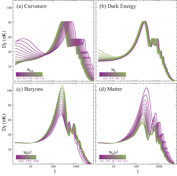 |
Plate 4. Sensitivity of the acoustic
temperature spectrum to four fundamental cosmological parameters (a)
the curvature as quantified by
|
The phenomenology of the acoustic peaks in the temperature and polarization
is essentially described by 4 observables and the initial conditions
[Hu et al, 1997].
These are the angular extents of the sound horizon
a
D*
/ s*,
the particle horizon at matter radiation equality
eq
keq
D* and the damping scale
d
kd
D* as well as the value of the baryon-photon
momentum density ratio R*.
a sets the
spacing between of the peaks;
eq and
d compete to
determine their
amplitude through radiation driving and diffusion damping.
R* sets the
baryon loading and, along with the potential well depths set by
eq,
fixes the modulation of the even and odd peak heights.
The initial conditions set the phase, or equivalently the location of
the first peak in units of
a, and an overall
tilt n in the power spectrum.
In the model of Plate 1, these numbers
are a = 301
(1 =
0.73a),
eq = 149,
d = 1332,
R* = 0.57 and n = 1 and in this family
of models the parameter sensitivity is approximately
[Hu et al, 2001]
 |
(24) |
and
R* / R*
1.0
b
h2 /
b
h2. Current observations indicate that
a = 304 ± 4,
eq = 168 ±
15, d = 1392
± 18, R* = 0.60 ± 0.06, and
n = 0.96 ± 0.04
([Knox et al, 2001];
see also
[Wang et al, 2001,
Pryke et al, 2001,
de Bernardis et al, 2001]),
if gravitational waves contributions
are subdominant and the reionization redshift is low as
assumed in the working cosmological model (see
Section 2.1).
The acoustic peaks therefore contain three rulers for the angular
diameter distance test for curvature, i.e. deviations from
tot = 1.
However contrary to popular belief, any one of these alone is not
a standard ruler whose absolute scale is known even in the
working cosmological model. This is reflected in the sensitivity of
these scales to other cosmological parameters.
For example, the dependence of
a on
m
h2 and hence the Hubble
constant is quite strong. But in combination with a measurement of
the matter-radiation ratio from
eq, this
degeneracy is broken.
The weaker degeneracy of
a on the baryons
can likewise be broken from a measurement of the baryon-photon ratio
R*. The damping scale
d provides an
additional consistency check on the implicit assumptions in the working
model, e.g. recombination and the energy contents
of the Universe during this epoch. What makes the peaks so valuable
for this test is that the rulers are standardizeable and contain
a built-in consistency check.
There remains a weak but perfect
degeneracy between
tot and
 because they both appear only in D*.
This is called the angular diameter distance degeneracy in the
literature and can readily be generalized to dark energy components beyond
the cosmological constant assumed here. Since the effect of
is
intrinsically so small, it only creates a correspondingly small
ambiguity in
tot for
reasonable values of
.
The down side is that dark energy can never be isolated through the peaks
alone since it only takes a small amount of curvature to mimic its effects.
The evidence for dark energy through the CMB comes about by allowing
for external information. The most important is the nearly overwhelming
direct evidence for
m < 1
from local structures in the Universe.
The second is the measurements of a relatively high Hubble constant
h 0.7;
combined with a relatively low
m
h2 that is preferred in the CMB data, it implies
m < 1
but at low significance currently.
because they both appear only in D*.
This is called the angular diameter distance degeneracy in the
literature and can readily be generalized to dark energy components beyond
the cosmological constant assumed here. Since the effect of
is
intrinsically so small, it only creates a correspondingly small
ambiguity in
tot for
reasonable values of
.
The down side is that dark energy can never be isolated through the peaks
alone since it only takes a small amount of curvature to mimic its effects.
The evidence for dark energy through the CMB comes about by allowing
for external information. The most important is the nearly overwhelming
direct evidence for
m < 1
from local structures in the Universe.
The second is the measurements of a relatively high Hubble constant
h 0.7;
combined with a relatively low
m
h2 that is preferred in the CMB data, it implies
m < 1
but at low significance currently.
The upshot is that precise measurements of the acoustic peaks
yield precise determinations of four fundamental parameters of the
working cosmological model:
b
h2,
m
h2, D*, and n. More
generally, the first three can be replaced by
a,
eq,
d and
R*
to extend these results to models where the underlying assumptions of the
working model are violated.
2 Recall that the comoving
scale k does not vary with time. At very early times, then, the
wavelengh k-1 is much larger than the horizon
.
Back.
 -
-
 plane)
generates linear polarization. Right: Polarization in the
plane)
generates linear polarization. Right: Polarization in the
 axis. The component of
the polarization
that is parallel or perpendicular to the wavevector k is called the
E-mode and the one at 45° angles is called the
B-mode.
axis. The component of
the polarization
that is parallel or perpendicular to the wavevector k is called the
E-mode and the one at 45° angles is called the
B-mode.