Copyright © 2002 by Annual Reviews. All rights reserved
| Annu. Rev. Astron. Astrophys. 2002. 40:
171-216 Copyright © 2002 by Annual Reviews. All rights reserved |


Once the acoustic peaks in the temperature and polarization power spectra have been scaled, the days of splendid isolation of cosmic microwave background theory, analysis and experiment will have ended. Beyond and beneath the peaks lies a wealth of information about the evolution of structure in the Universe and its origin in the early universe. As CMB photons traverse the large scale structure of the Universe on their journey from the recombination epoch, they pick up secondary temperature and polarization anisotropies. These depend on the intervening dark matter, dark energy, baryonic gas density and temperature distributions, and even the existence of primordial gravity waves, so the potential payoff of their detection is enormous. The price for this extended reach is the loss of the ability both to make precise predictions, due to uncertain and/or non-linear physics, and to make precise measurements, due to the cosmic variance of the primary anisotropies and the relatively greater importance of galactic and extragalactic foregrounds.
We begin in Section 4.1 with a discussion of the matter power spectrum to set the framework for the discussion of secondary anisotropies. Secondaries can be divided into two classes: those due to gravitational effects and those induced by scattering off of electrons. The former are treated in Section 4.2 and the latter in Section 4.3. Secondary anisotropies are often non-Gaussian, so they show up not only in the power spectra of Section 2, but in higher point functions as well. We briefly discuss non-Gaussian statistics in Section 4.4. All of these topics are subjects of current research to which this review can only serve as introduction.
The same balance between pressure and gravity that is responsible for acoustic oscillations determines the power spectrum of fluctuations in the non-relativistic matter. This relationship is often obscured by focussing on the density fluctuations in the pressureless cold dark matter itself and we so we will instead consider the matter power spectrum from the perspective of the Newtonian potential.
4.1.1 PHYSICAL DESCRIPTION
After recombination, without the pressure of the photons, the baryons
simply fall into the Newtonian potential wells with the cold dark matter,
an event usually referred to as the end of the Compton drag epoch.
We claimed in
Section 3.5 that above the horizon at
matter-radiation equality the potentials are nearly constant.
This follows from the dynamics: where pressure gradients are
negligible, infall into some initial potential causes a potential flow of
vtot ~ (k
 )
)
 i
[see Equation (19)] and causes density enhancements by continuity of
i
[see Equation (19)] and causes density enhancements by continuity of
 tot ~ -
(k
)
vtot ~ - (k
)2
i. The
Poisson equation says that the potential at this later time
~ - (k
)-2
tot ~
i so that
this rate of growth is exactly right to keep the potential constant.
Formally, this Newtonian argument only applies in general relativity
for a particular choice of coordinates
[Bardeen, 1980],
but the rule of thumb
is that if what is driving the expansion (including spatial curvature)
can also cluster unimpeded by pressure,
the gravitational potential will remain constant.
tot ~ -
(k
)
vtot ~ - (k
)2
i. The
Poisson equation says that the potential at this later time
~ - (k
)-2
tot ~
i so that
this rate of growth is exactly right to keep the potential constant.
Formally, this Newtonian argument only applies in general relativity
for a particular choice of coordinates
[Bardeen, 1980],
but the rule of thumb
is that if what is driving the expansion (including spatial curvature)
can also cluster unimpeded by pressure,
the gravitational potential will remain constant.
Because the potential is constant in
the matter dominated epoch, the large-scale observations of COBE set
the overall amplitude of the potential power spectrum today. Translated
into density, this is the well-known COBE normalization. It is usually
expressed in terms of
H, the matter
density perturbation at the Hubble scale today.
Since the observed temperature fluctuation is approximately
/ 3,
 |
(25) |
where the second equality follows from the Poisson equation
in a fully matter dominated universe with
 m = 1.
The observed COBE fluctuation of
m = 1.
The observed COBE fluctuation of
 T
T
 28µK
[Smoot et al, 1992]
implies H
2 ×
10-5. For corrections for
m < 1
where the potential decays because the dominant driver of
the expansion cannot cluster, see
[Bunn & White, 1997].
28µK
[Smoot et al, 1992]
implies H
2 ×
10-5. For corrections for
m < 1
where the potential decays because the dominant driver of
the expansion cannot cluster, see
[Bunn & White, 1997].
On scales below the horizon at matter-radiation equality,
we have seen in Section 3.5 that pressure
gradients from the acoustic oscillations themselves impede the
clustering of the dominant component, i.e. the photons, and lead to
decay in the potential. Dark matter density perturbations
remain but grow only logarithmically from their value at horizon crossing,
which (just as for large scales) is approximately the initial potential,
m
-
i.
The potential for modes that have entered the horizon already will
therefore be suppressed by
 -
m /
k2 ~
i /
k2 at matter domination
(neglecting the logarithmic growth)
again according to the Poisson equation. The ratio of
at late times to
its initial
value is called the transfer function. On large scales, then, the
transfer function is close to one, while it falls off as
k-2 on small scales. If the baryons fraction
-
m /
k2 ~
i /
k2 at matter domination
(neglecting the logarithmic growth)
again according to the Poisson equation. The ratio of
at late times to
its initial
value is called the transfer function. On large scales, then, the
transfer function is close to one, while it falls off as
k-2 on small scales. If the baryons fraction
 b
/ m
is substantial, baryons alter
the transfer function in two ways. First their inability
to cluster below the sound horizon
causes further decay in the potential between matter-radiation
equality and the end of the Compton drag epoch. Secondly the
acoustic oscillations in the baryonic velocity field kinematically cause
acoustic wiggles in the transfer function
[Hu & Sugiyama, 1996].
These wiggles
in the matter power spectrum are related to the acoustic peaks
in the CMB spectrum like twins separated at birth and are actively
being pursued by the largest galaxy surveys
[Percival et al, 2001].
For fitting formulae for the transfer function that include these
effects see
[Eisenstein & Hu, 1998].
b
/ m
is substantial, baryons alter
the transfer function in two ways. First their inability
to cluster below the sound horizon
causes further decay in the potential between matter-radiation
equality and the end of the Compton drag epoch. Secondly the
acoustic oscillations in the baryonic velocity field kinematically cause
acoustic wiggles in the transfer function
[Hu & Sugiyama, 1996].
These wiggles
in the matter power spectrum are related to the acoustic peaks
in the CMB spectrum like twins separated at birth and are actively
being pursued by the largest galaxy surveys
[Percival et al, 2001].
For fitting formulae for the transfer function that include these
effects see
[Eisenstein & Hu, 1998].
4.1.2 COSMOLOGICAL IMPLICATIONS
The combination of the COBE normalization, the matter transfer function
and the near scale-invariant initial spectrum of fluctuations
tells us that by the present fluctuations in the cold dark matter
or baryon density fields will have gone non-linear for all scales
k  10-1 hMpc-1.
It is a great triumph of the standard cosmological paradigm that
there is just enough growth between z*
103 and
z = 0 to explain structures in the Universe across a wide range
of scales.
10-1 hMpc-1.
It is a great triumph of the standard cosmological paradigm that
there is just enough growth between z*
103 and
z = 0 to explain structures in the Universe across a wide range
of scales.
In particular, since this non-linear scale
also corresponds to galaxy clusters and measurements of
their abundance yields a robust measure of the power near this
scale for a given matter density
m.
The agreement between the COBE normalization and the cluster abundance
at low
m ~ 0.3 -
0.4 and the observed Hubble constant
h = 0.72 ± 0.08
[Freedman et al, 2001]
was pointed out immediately following the COBE result (e.g.
[White et al, 1993,
Bartlett & Silk, 1993])
and is one of the strongest pieces of evidence for the
parameters in the working cosmological model
[Ostriker & Steinhardt, 1995,
Krauss & Turner, 1995].
More generally, the comparison between large-scale structure and the CMB is important in that it breaks degeneracies between effects due to deviations from power law initial conditions and the dynamics of the matter and energy contents of the Universe. Any dynamical effect that reduces the amplitude of the matter power spectrum corresponds to a decay in the Newtonian potential that boosts the level of anisotropy (see Section 3.5 and Section 4.2.1). Massive neutrinos are a good example of physics that drives the matter power spectrum down and the CMB spectrum up.
The combination is even more fruitful in the relationship between
the acoustic peaks and the baryon wiggles in the matter power spectrum.
Our knowledge of the physical distance between adjacent
wiggles provides the ultimate standard candle for cosmology
[Eisenstein et al, 1998].
For example, at very low z, the radial distance out to a galaxy is
cz / H0. The unit of distance is therefore
h-1 Mpc, and a knowledge
of the true physical distance corresponds to a determination of h.
At higher redshifts, the radial distance depends sensitively on the
background cosmology (especially the dark energy), so a future measurement
of baryonic wiggles at z ~ 1 say would be a powerful test of dark
energy models. To a lesser extent,
the shape of the transfer function, which mainly depends on the
matter-radiation scale in h Mpc-1, i.e.
m h,
is another standard ruler (see e.g.
[Tegmark et al, 2001] for
a recent assessment), more heralded than the wiggles, but less robust
due to degeneracy with other cosmological parameters.
For scales corresponding to
k
10-1 h Mpc-1, density fluctuations
are non-linear by the present. Numerical N-body simulations show
that the dark matter is bound up in a hierarchy of virialized structures
or halos (see
[Bertschinger, 1998]
for a review).
The statistical properties of the dark matter and the dark matter halos
have been extensively studied in the working cosmological model. Less
certain are the properties of the baryonic gas. We shall see that both
enter into the consideration of secondary CMB anisotropies.
4.2. Gravitational Secondaries
Gravitational secondaries arise from two sources: the differential redshift from time-variable metric perturbations [Sachs & Wolfe, 1967] and gravitational lensing. There are many examples of the former, one of which we have already encountered in Section 3.8 in the context of potential decay in the radiation dominated era. Such gravitational potential effects are usually called the integrated Sachs-Wolfe (ISW) effect in linear perturbation theory (Section 4.2.1), the Rees-Sciama (Section 4.2.2) effect in the non-linear regime, and the gravitational wave effect for tensor perturbations (Section 4.2.3). Gravitational waves and lensing also produce B-modes in the polarization (see Section 3.7) by which they may be distinguished from acoustic polarization.
4.2.1 ISW EFFECT
As we have seen in the previous section, the potential on a given scale
decays whenever the expansion
is dominated by a component whose effective density is
smooth on that scale. This occurs at late times in an
m < 1
model at the end of matter domination and
the onset dark energy (or spatial curvature) domination.
If the potential decays between the time a photon falls into
a potential well and when it climbs out it gets a boost in temperature
of
due to the differential
gravitational redshift and
-
 due to an accompanying
contraction of the wavelength (see Section 3.3).
due to an accompanying
contraction of the wavelength (see Section 3.3).
Potential decay due to residual radiation was introduced in Section 3.8, but that due to dark energy or curvature at late times induces much different changes in the anisotropy spectrum. What makes the dark energy or curvature contributions different from those due to radiation is the longer length of time over which the potentials decay, on order the Hubble time today. Residual radiation produces its effect quickly, so the distance over which photons feel the effect is much smaller than the wavelength of the potential fluctuation. Recall that this meant that jl(kD) in the integral in Equation (23) could be set to jl(kD*) and removed from the integral. The final effect then is proportional to jl(kD*) and adds in phase with the monopole.
The ISW projection, indeed the projection of all secondaries,
is much different (see Plate 3).
Since the duration of the potential change is much
longer, photons typically travel through many peaks and troughs of
the perturbation. This cancellation implies that many modes
have virtually no impact on the photon temperature. The only modes which
do have an impact are those with wavevectors
perpendicular to the line of sight, so that along the line of sight
the photon does not pass through crests and troughs. What fraction of
the modes contribute to the effect then? For a given wavenumber k
and line of sight instead of the full spherical shell at radius
4 k2
dk, only the ring
2kdk with
k
k2
dk, only the ring
2kdk with
k  n
participate. Thus, the anisotropy induced is suppressed by a
factor of k (or
n
participate. Thus, the anisotropy induced is suppressed by a
factor of k (or
 = kD in angular space).
Mathematically, this arises in the line-of-sight integral of
Equation (23) from the integral over the oscillatory Bessel function
= kD in angular space).
Mathematically, this arises in the line-of-sight integral of
Equation (23) from the integral over the oscillatory Bessel function
 dxj (x)
( /
2)1/2
(see also Plate 3).
dxj (x)
( /
2)1/2
(see also Plate 3).
The ISW effect thus generically shows up only at the lowest
's in the power spectrum
([Kofman & Starobinskii, 1985]).
This spectrum is shown in
Plate 5. Secondary anisotropy
predictions in this figure are for a model with
tot = 1,
 =
2/3, b
h2 = 0.02,
m
h2 = 0.16, n = 1,
zri = 7 and inflationary energy scale
Ei << 1016 GeV.
The ISW effect is especially important in that it is extremely sensitive
to the dark energy: its amount, equation of state and clustering properties
[Coble et al, 1997,
Caldwell et al, 1998,
Hu, 1998].
Unfortunately, being confined to the low multipoles,
the ISW effect suffers severely from the cosmic variance in
Equation (4) in its detectability.
Perhaps more promising is its correlation with other tracers of
the gravitational potential (e.g. X-ray background
[Boughn et al, 1998]
and gravitational lensing, see Section 4.2.4).
=
2/3, b
h2 = 0.02,
m
h2 = 0.16, n = 1,
zri = 7 and inflationary energy scale
Ei << 1016 GeV.
The ISW effect is especially important in that it is extremely sensitive
to the dark energy: its amount, equation of state and clustering properties
[Coble et al, 1997,
Caldwell et al, 1998,
Hu, 1998].
Unfortunately, being confined to the low multipoles,
the ISW effect suffers severely from the cosmic variance in
Equation (4) in its detectability.
Perhaps more promising is its correlation with other tracers of
the gravitational potential (e.g. X-ray background
[Boughn et al, 1998]
and gravitational lensing, see Section 4.2.4).
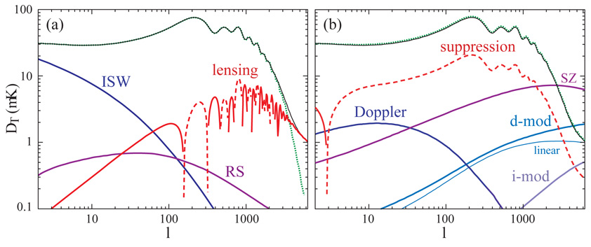 |
Plate 5. Secondary anisotropies. (a)
Gravitational secondaries: ISW, lensing and Rees-Sciama (moving halo)
effects. (b) Scattering secondaries: Doppler, density
( |
This type of cancellation behavior and corresponding suppression of
small scale fluctuations is a common feature of secondary
temperature and polarization anisotropies from large-scale structure
and is quantified by the Limber equation
[Limber, 1954]
and its CMB generalization
[Hu & White, 1996,
Hu, 2000a].
It is the central reason why secondary anisotropies tend to be smaller
than the primary ones from
z*
103
despite the intervening growth of structure.
4.2.2. REES-SCIAMA AND MOVING HALO EFFECTS The ISW effect is linear in the perturbations. Cancellation of the ISW effect on small scales leaves second order and non-linear analogues in its wake [Rees & Sciama, 1968]. From a single isolated structure, the potential along the line of sight can change not only from evolution in the density profile but more importantly from its bulk motion across the line of sight. In the context of clusters of galaxies, this is called the moving cluster effect [Birkinshaw & Gull, 1983]. More generally, the bulk motion of dark matter halos of all masses contribute to this effect [Tuluie & Laguna, 1995, Seljak, 1996b], and their clustering gives rise to a low level of anisotropies on a range of scales but is never the leading source of secondary anisotropies on any scale (see Plate 5a).
4.2.3. GRAVITATIONAL WAVES
A time-variable tensor metric perturbation similarly leaves an imprint in
the temperature anisotropy
[Sachs & Wolfe, 1967].
A tensor metric perturbation
can be viewed as a standing gravitational wave and produces a quadrupolar
distortion in the spatial metric. If its
amplitude changes, it leaves a quadrupolar distortion in
the CMB temperature distribution
[Polnarev, 1985].
Inflation predicts a nearly scale-invariant spectrum of gravitational
waves. Their amplitude depends strongly on the
energy scale of inflation,
3
(power
Ei4
[Rubakov et al, 1982,
Fabbri & Pollock, 1983])
and its relationship to the curvature fluctuations discriminates between
particular
models for inflation. Detection of gravitational waves in the CMB therefore
provides our best hope to study the particle physics of inflation.
Gravitational waves, like scalar fields,
obey the Klein-Gordon equation in a flat universe
and their amplitudes begin oscillating and decaying once the
perturbation crosses the horizon. While this process occurs
even before recombination,
rapid Thomson scattering destroys any quadrupole anisotropy that
develops (see Section 3.6). This
fact dicates the general structure of the contributions
to the power spectrum (see Figure 4, left panel):
they are enhanced at = 2
the present quadrupole
and sharply suppressed at multipole larger than that of the first peak
[Abbott & Wise, 1984,
Starobinskii, 1985,
Crittenden et al, 1993].
As is the case for the ISW effect, confinement to the low
multipoles means that the isolation of gravitational waves is severely
limited by cosmic variance.
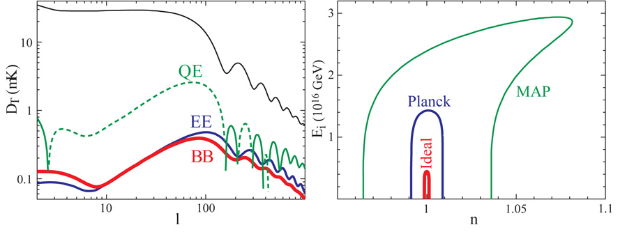 |
Figure 4. Gravitational waves and the
energy scale of
inflation Ei. Left: temperature and polarization
spectra from an initial scale invariant gravitational wave spectrum with
power |
The signature of gravitational waves in the polarization is more distinct. Because gravitational waves cause a quadrupole temperature anisotropy at the end of recombination, they also generate a polarization. The quadrupole generated by a gravitational wave has its main angular variation transverse to the wavevector itself [Hu & White, 1997a]. The resulting polarization that results has components directed both along or orthogonal to the wavevector and at 45° degree angles to it. Gravitational waves therefore generate a nearly equal amount of E and B mode polarization when viewed at a distance that is much greater than a wavelength of the fluctuation [Kamionkowski et al, 1997, Zaldarriaga & Seljak, 1997]. The B-component presents a promising means of measuring the gravitational waves from inflation and hence the energy scale of inflation (see Figure 4, right panel). Models of inflation correspond to points in the n, Ei plane [Dodelson et al, 1997]. Therefore, the anticipated constraints will discriminate among different models of inflation, probing fundamental physics at scales well beyond those accessible in accelerators.
4.2.4. GRAVITATIONAL LENSING
The gravitational potentials of large-scale structure also lens the
CMB photons. Since lensing conserves surface brightness, it only
affects anisotropies and hence is second order in perturbation theory
[Blanchard & Schneider, 1987].
The photons are deflected according to the angular gradient of
the potential projected along the line of sight with a weighting of
2(D* - D) /
(D* D). Again the cancellation of
parallel modes implies that it is mainly the large-scale potentials
that are responsible for deflections.
Specifically, the angular gradient
of the projected potential peaks at a multipole
~ 60 corresponding
to scales of a k ~ few 10-2 Mpc-1
[Hu, 2000b].
The deflections are therefore coherent below the degree scale. The
coherence of the deflection should not be
confused with its rms value which in the model of
Plate 1 has
a value of a few arcminutes.
This large coherence and small amplitude ensures that linear theory in
the potential is sufficient to describe the main effects of
lensing. Since lensing is a one-to-one mapping of the source
and image planes it simply distorts the images formed from the
acoustic oscillations in accord with the deflection angle. This
warping naturally also distorts the mapping of physical scales
in the acoustic peaks to angular scales
Section 3.8 and hence
smooths features in the temperature and polarization
[Seljak, 1996a].
The smoothing scale is the coherence scale of the deflection angle
60 and
is sufficiently wide to alter the acoustic peaks with
~ 300.
The contributions, shown in
Plate 5a are therefore
negative (dashed) on scales corresponding to the peaks.
For the polarization, the remapping not only smooths the acoustic power spectrum but actually generates B-mode polarization (see Plate 1 and [Zaldarriaga & Seljak, 1998]). Remapping by the lenses preserves the orientation of the polarization but warps its spatial distribution in a Gaussian random fashion and hence does not preserve the symmetry of the original E-mode. The B-modes from lensing sets a detection threshold for gravitational waves for a finite patch of sky [Hu, 2001b].
Gravitational lensing also generates a small amount of power in the anisotropies on its own but this is only noticable beyond the damping tail where diffusion has destroyed the primary anisotropies (see Plate 5). On these small scales, the anisotropy of the CMB is approximately a pure gradient on the sky and the inhomogeneous distribution of lenses introduces ripples in the gradient on the scale of the lenses [Seljak & Zaldarriaga, 2000]. In fact the moving halo effect of Section 4.2.2 can be described as the gravitational lensing of the dipole anisotropy due to the peculiar motion of the halo [Birkinshaw & Gull, 1983].
Because the lensed CMB distribution is not linear in the fluctuations, it is not completely described by changes in the power spectrum. Much of the recent work in the literature has been devoted to utilizing the non-Gaussianity to isolate lensing effects [Bernardeau, 1997, Bernardeau, 1998, Zaldarriaga & Seljak, 1999, Zaldarriaga, 2000] and their cross-correlation with the ISW effect [Goldberg & Spergel, 1999, Seljak & Zaldarriaga, 1999]. In particular, there is a quadratic combination of the anisotropy data that optimally reconstructs the projected dark matter potentials for use in this cross-correlation [Hu, 2001c]. The cross correlation is especially important in that in a flat universe it is a direct indication of dark energy and can be used to study the properties of the dark energy beyond a simple equation of state [Hu, 2001b].
From the observations both of the lack of of a Gunn-Peterson trough
[Gunn & Peterson, 1965]
in quasar spectra and its preliminary detection
[Becker et al, 2001],
we know that hydrogen was reionized at zri
6. This is
thought to occur through the ionizing radiation of the first generation of
massive stars (see e.g.
[Loeb & Barkana, 2001]
for a review). The consequent
recoupling of CMB photons to the baryons causes a few percent of them
to be rescattered. Linearly, rescattering induces three changes to the
photon distribution: suppression of primordial anisotropy, generation of
large angle polarization, and a large angle Doppler effect. The latter
two are suppressed on small scales by the cancellation highlighted in
Section 4.2.1. Non-linear
effects can counter this suppression; these are the subject of active
research and are outlined in Section 4.3.4.
4.3.1. PEAK SUPPRESSION
Like scattering before recombination, scattering at late times
suppresses anisotropies in the distribution that
have already formed. Reionization therefore suppresses the amplitude
of the acoustic peaks by the fraction of photons rescattered,
approximately the optical depth
~  ri (see
Plate 5b,
dotted line and negative, dashed line, contributions corresponding to
|
T2|1/2 between the
zri = 7 and zri = 0 models).
Unlike the plasma before recombination, the medium is optically thin
and so the mean free path and diffusion length of the
photons is of order the horizon itself. New acoustic oscillations cannot
form. On scales approaching
the horizon at reionization, inhomogeneities have yet to be converted
into anisotropies (see Section 3.8)
and so large angle fluctuations
are not suppressed. While these effects are relatively large compared
with the expected precision of future experiments, they mimic a
change in the overall normalization of fluctuations except at the
lowest, cosmic variance limited, multipoles.
ri (see
Plate 5b,
dotted line and negative, dashed line, contributions corresponding to
|
T2|1/2 between the
zri = 7 and zri = 0 models).
Unlike the plasma before recombination, the medium is optically thin
and so the mean free path and diffusion length of the
photons is of order the horizon itself. New acoustic oscillations cannot
form. On scales approaching
the horizon at reionization, inhomogeneities have yet to be converted
into anisotropies (see Section 3.8)
and so large angle fluctuations
are not suppressed. While these effects are relatively large compared
with the expected precision of future experiments, they mimic a
change in the overall normalization of fluctuations except at the
lowest, cosmic variance limited, multipoles.
4.3.2. LARGE-ANGLE POLARIZATION
The rescattered radiation becomes polarized since, as discussed
in Section 3.8 temperature inhomogeneities,
become anisotropies by projection, passing through quadrupole anisotropies
when the perturbations are on the horizon scale at any given time.
The result is a bump in the power spectrum of the E-polarization on
angular scales corresponding to the horizon at reionization (see
Plate 1). Because of the low optical depth of
reionization and the finite range of scales that contribute to the
quadrupole, the polarization contributions are on the order of tenths of
µK on
scales of ~ few. In a
perfect, foreground free world, this
is not beyond the reach of experiments and can be used to isolate
the reionization epoch
[Hogan et al, 1982,
Zaldarriaga et al, 1997].
As in the ISW effect, cancellation of contributions along the line of
sight guarantees a sharp suppression of contributions at higher
multipoles in linear theory.
Spatial modulation of the optical depth due to density and ionization
(see Section 4.3.4) does produce higher order
polarization but at an entirely negligible level in most models
[Hu, 2000a].
4.3.3. DOPPLER EFFECT
Naively, velocity fields of order v ~ 10-3 (see e.g.
[Strauss & Willick, 1995]
for a review) and optical depths of
a few percent would imply a Doppler effect that rivals the acoustic peaks
themselves. That this is not the case is the joint consequence of the
cancellation described in Section 4.2.1 and the
fact that the acoustic peaks are not "Doppler peaks"
(see Section 3.8).
Since the Doppler effect comes from the peculiar
velocity along the line of sight, it retains no contributions from linear
modes with wavevectors perpendicular to the line of sight. But as we
have seen, these are the only modes that survive cancellation (see
Plate 3 and
[Kaiser, 1984]).
Consequently, the Doppler
effect from reionization is strongly suppressed and is entirely
negligible below
~ 102
unless the optical depth in the reionization epoch approaches
unity (see Plate 5b).
4.3.4. MODULATED DOPPLER EFFECTS The Doppler effect can survive cancellation if the optical depth has modulations in a direction orthogonal to the bulk velocity. This modulation can be the result of either density or ionization fluctuations in the gas. Examples of the former include the effect in clusters, and linear as well as non-linear large-scale structures.
CLUSTER MODULATION: The strongly non-linear modulation provided by the presence of a galaxy cluster and its associated gas leads to the kinetic Sunyaev-Zel'dovich effect. Cluster optical depths on order 10-2 and peculiar velocities of 10-3 imply signals in the 10-5 regime in individual arcminute-scale clusters, which are of course rare objects. While this signal is reasonably large, it is generally dwarfed by the thermal Sunyaev-Zel'dovich effect (see Section 4.3.5) and has yet to be detected with high significance (see [Carlstrom et al, 2001] and references therein). The kinetic Sunyaev-Zel'dovich effect has negligible impact on the power spectrum of anisotropies due to the rarity of clusters and can be included as part of the more general density modulation.
LINEAR MODULATION:
At the opposite extreme, linear density fluctuations modulate
the optical depth and give rise to a Doppler effect as pointed out by
[Ostriker & Vishniac, 1986]
and calculated by
[Vishniac, 1987]
(see also
[Efstathiou & Bond, 1987]).
The result is a signal at the µK level peaking
at ~ few
× 103 that increases roughly logarithmically
with the reionization redshift (see Plate 5b).
GENERAL DENSITY MODULATION:
Both the cluster and linear modulations are limiting cases of the more
general effect of density modulation by the large scale structure of
the Universe. For the low reionization redshifts currently expected
(zri
6 - 7) most of the effect comes neither from clusters
nor the linear regime but intermediate scale dark matter halos.
An upper limit to the total effect can be obtained by assuming the
gas traces the dark matter
[Hu, 2000a]
and implies signals on the order of
T ~ few
µK at
> 103 (see
Plate 5b). Based on simulations, this assumption
should hold in the outer profiles of
halos [Pearce et al, 2001,
Lewis et al, 2000]
but gas pressure will tend to smooth out the distribution in the cores
of halos and reduce small scale contributions. In the absence of
substantial cooling and star formation, these net effects
can be modeled under the assumption of hydrostatic equilibrium
[Komatsu & Seljak, 2001]
in the halos and included in a halo approach to the gas distribution
[Cooray, 2001].
IONIZATION MODULATION:
Finally, optical depth modulation can also come from variations
in the ionization fraction
[Aghanim et al, 1996,
Gruzinov & Hu, 1998,
Knox et al, 1998].
Predictions for this effect are the most
uncertain as it involves both the formation of the first ionizing
objects and the subsequent radiative transfer of the ionizing radiation
[Bruscoli et al, 2000,
Benson et al, 2001].
It is however unlikely to dominate the density modulated effect except
perhaps at very high multipoles
~ 104 (crudely
estimated, following
[Gruzinov & Hu, 1998],
in Plate 5b).
4.3.5. SUNYAEV-ZEL'DOVICH EFFECT
Internal motion of the gas in dark matter halos also give rise
to Doppler shifts in the CMB photons. As in the linear Doppler
effect, shifts that are first order in the velocity are canceled
as photons scatter off of electrons moving in different directions.
At second order in the velocity, there is a residual effect. For
clusters of galaxies where the temperature of the gas can reach
Te ~ 10 keV,
the thermal motions are a substantial fraction of the speed of light
vrms = (3Te /
me)1/2 ~ 0.2. The second order effect
represents a net transfer of energy between the hot electron
gas and the cooler CMB and leaves a spectral distortion in the CMB
where photons on the Rayleigh-Jeans side are transferred to the Wien
tail. This effect is called the thermal Sunyaev-Zel'dovich (SZ) effect
[Sunyaev & Zel'dovich, 1972].
Because the net effect is of order
cluster
Te / me
ne
Te, it is a probe of the gas pressure.
Like all CMB effects, once imprinted, distortions
relative to the redshifting background temperature remain unaffected
by cosmological dimming, so one might hope to find clusters at high
redshift using the SZ effect. However, the main effect comes from the
most massive clusters because of the strong temperature weighting
and these have formed only recently in the standard cosmological model.
Great strides have recently been made in observing the SZ effect in individual clusters, following pioneering attempts that spanned two decades [Birkinshaw, 1999]. The theoretical basis has remained largely unchanged save for small relativistic corrections as Te / me approches unity. Both developements are comprehensively reviewed in [Carlstrom et al, 2001]. Here we instead consider its implications as a source of secondary anisotropies.
The SZ effect from clusters provides the most substantial contribution to
temperature anisotropies beyond the damping tail. On scales much larger
than an arcminute where clusters are unresolved, contributions to
the power spectrum appear as uncorrelated shot noise
(C = const. or
T
). The additional
contribution due to the
spatial correlation of clusters turns out to be almost negligible in
comparison due to the rarity of clusters
[Komatsu & Kitayama, 1999].
Below this scale, contributions turn
over as the clusters become resolved. Though there has been much
recent progress in simulations
[Refregier et al, 2000,
Seljak et al, 2001,
Springel et al, 2001]
dynamic range still presents a serious limitation.
Much recent work has been devoted to semi-analytic modeling following the technique of [Cole & Kaiser, 1988], where the SZ correlations are described in terms of the pressure profiles of clusters, their abundance and their spatial correlations [now commonly referred to an application of the "halo model" see [Komatsu & Kitayama, 1999, Atrio-Barandela & Mücket, 1999, Cooray, 2001, Komatsu & Seljak, 2001]]. We show the predictions of a simplified version in Plate 5b, where the pressure profile is approximated by the dark matter haloprofile and the virial temperature of halo. While this treatment is comparatively crude, the inaccuracies that result are dwarfed by "missing physics" in both the simulations and more sophisticated modelling, e.g. the non-gravitational sources and sinks of energy that change the temperature and density profile of the cluster, often modeled as a uniform "preheating" of the intercluster medium [Holder & Carlstrom, 2001].
Although the SZ effect is expected to dominate the power spectrum of secondary anisotropies, it does not necessarily make the other secondaries unmeasurable or contaminate the acoustic peaks. Its distinct frequency signature can be used to isolate it from other secondaries (see e.g. [Cooray et al, 2000]). Additionally, it mainly comes from massive clusters which are intrinsically rare. Hence contributions to the power spectrum are non-Gaussian and concentrated in rare, spatially localized regions. Removal of regions identified as clusters through X-rays and optical surveys or ultimately high resolution CMB maps themselves can greatly reduce contributions at large angular scales where they are unresolved [Persi et al, 1995, Komatsu & Kitayama, 1999].
As we have seen, most of the secondary anisotropies are not linear in nature and hence produce non-Gaussian signatures. Non-Gaussianity in the lensing and SZ signals will be important for their isolation. The same is true for contaminants such as galactic and extragalactic foregrounds. Finally the lack of an initial non-Gaussianity in the fluctuations is a testable prediction of the simplest inflationary models [Guth & Pi, 1985, Bardeen et al, 1983]. Consequently, non-Gaussianity in the CMB is currently a very active field of research. The primary challenge in studies of non-Gaussianity is in choosing the statistic that quantifies it. Non-Gaussianity says what the distribution is not, not what it is. The secondary challenge is to optimize the statistic against the Gaussian "noise" of the primary anisotropies and instrumental or astrophysical systematics.
Early theoretical work on the bispectrum, the harmonic analogue of the three point function addressed its detectability in the presence of the cosmic variance of the Gaussian fluctuations [Luo, 1994] and showed that the inflationary contribution is not expected to be detectable in most models ([Allen et al, 1987, Falk et al, 1993]). The bispectrum is defined by a triplet of multipoles, or configuration, that defines a triangle in harmonic space. The large cosmic variance in an individual configuration is largely offset by the great number of possible triplets. Interest was spurred by reports of significant signals in specific bispectrum configurations in the COBE maps [Ferreira et al, 1998] that turned out to be due to systematic errors [Banday et al, 2000]. Recent investigations have focussed on the signatures of secondary anisotropies [Goldberg & Spergel, 1999, Cooray & Hu, 2000]. These turn out to be detectable with experiments that have both high resolution and angular dynamic range but require the measurement of a wide range of configurations of the bispectrum. Data analysis challenges for measuring the full bispectrum largely remain to be addressed (c.f. [Heavens, 1998, Spergel & Goldberg, 1999, Phillips & Kogut, 2001]).
The trispectrum, the harmonic analogue of the four point function, also has advantages for the study of secondary anisotropies. Its great number of configurations are specified by a quintuplet of multipoles that correspond to the sides and diagonal of a quadrilateral in harmonic space [Hu, 2001a]. The trispectrum is important in that it quantifies the covariance of the power spectrum across multipoles that is often very strong in non-linear effects, e.g. the SZ effect [Cooray, 2001]. It is also intimately related to the power spectra of quadratic combinations of the temperature field and has been applied to study gravitational lensing effects [Bernardeau, 1997, Zaldarriaga, 2000, Hu, 2001a].
The bispectrum and trispectrum quantify non-Gaussianity in harmonic space, and have clear applications for secondary anisotropies. Tests for non-Gaussianity localized in angular space include the Minkowski functionals (including the genus) [Winitzki & Kosowsky, 1997], the statistics of temperature extrema [Kogut et al, 1996], and wavelet coefficients [Aghanim & Forni, 1999]. These may be more useful for examining foreground contamination and trace amounts of topological defects.
3 Ei4
 V(
V( ), the
potential
energy density associated with the scalar field(s) driving inflation.
Back.
), the
potential
energy density associated with the scalar field(s) driving inflation.
Back.