4. IONISATION BALANCE

In order to calculate the X-ray emission or absorption from a plasma, apart from the physical conditions also the ion concentrations must be known. These ion concentrations can be determined by solving the equations for ionisation balance (or in more complicated cases by solving the time-dependent equations). A basic ingredient in these equations are the ionisation and recombination rates, that we discussed in the previous section. Here we consider three of the most important cases: collisional ionisation equilibrium, non-equilibrium ionisation and photoionisation equilibrium.

4.1. Collisional Ionisation Equilibrium (CIE)

The simplest case is a plasma in collisional ionisation equilibrium (CIE). In this case one assumes that the plasma is optically thin for its own radiation, and that there is no external radiation field that affects the ionisation balance.

Photo-ionisation and Compton ionisation therefore can be neglected in the case of CIE. This means that in general each ionisation leads to one additional free electron, because the direct ionisation and excitation-autoionisation processes are most efficient for the outermost atomic shells. The relevant ionisation processes are collisional ionisation and excitation-autoionisation, and the recombination processes are radiative recombination and dielectronic recombination. Apart from these processes, at low temperatures also charge transfer ionisation and recombination are important.

We define R_z as the total recombination rate of an ion with charge z to charge z - 1, and I_z as the total ionisation rate for charge z to z + 1. Ionisation equilibrium then implies that the net change of ion concentrations n_z should be zero:

(22)

and in particular for z = 0 one has

(23)

(a neutral atom cannot recombine further and it cannot be created by ionisation). Next an arbitrary value for n₀ is chosen, and (23) is solved:

(24)

This is substituted into (22) which now can be solved. Using induction, it follows that

(25)

Finally everything is normalised by demanding that

(26)

where n_element is the total density of the element, determined by the total plasma density and the chemical abundances.

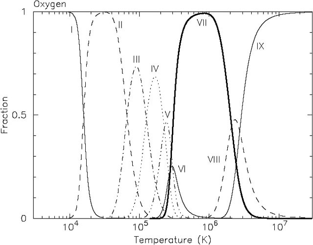
Examples of plasmas in CIE are the Solar corona, coronae of stars, the hot intracluster medium, the diffuse Galactic ridge component. Fig. 7 shows the ion fractions as a function of temperature for two important elements.

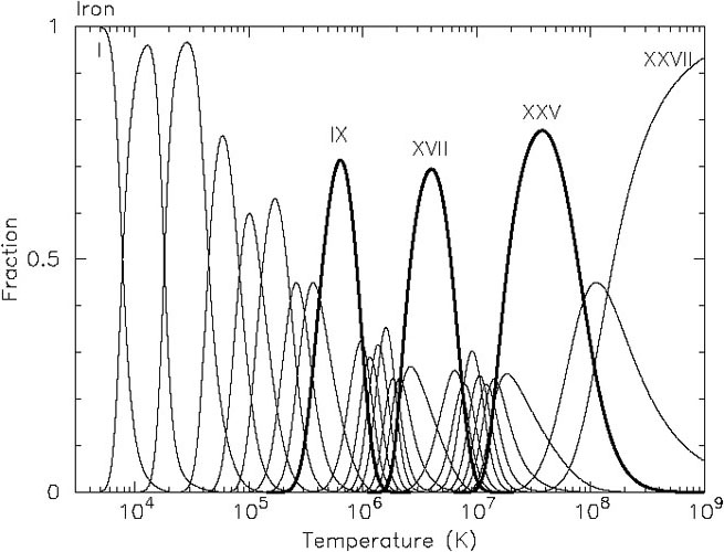Figure 7. Ion concentration of oxygen ions (left panel) and iron ions (right panel) as a function of temperature in a plasma in Collisional Ionisation Equilibrium (CIE). Ions with completely filled shells are indicated with thick lines: the He-like ions O VII and Fe XXV, the Ne-like Fe XVII and the Ar-like Fe IX; note that these ions are more prominent than their neighbours.

4.2. Non-Equilibrium Ionisation (NEI)

The second case that we discuss is non-equilibrium ionisation (NEI). This situation occurs when the physical conditions of the source, like the temperature, suddenly change. A shock, for example, can lead to an almost instantaneous rise in temperature. However, it takes a finite time for the plasma to respond to the temperature change, as ionisation balance must be recovered by collisions. Similar to the CIE case we assume that photoionisation can be neglected. For each element with nuclear charge Z we write:

(27)

where is a vector of length Z + 1 that contains the ion concentrations, and which is normalised according to Eqn. 26. The transition matrix A is a (Z + 1) × (Z + 1) matrix given by

We can write the equation in this form because both ionisations and recombinations are caused by collisions of electrons with ions. Therefore we have the uniform scaling with n_e. In general, the set of equations (27) must be solved numerically. The time evolution of the plasma can be described in general well by the parameter

(28)

The integral should be done over a co-moving mass element. Typically, for most ions equilibrium is reached for U ~ 10¹⁸ m^-3s. We should mention here, however, that the final outcome also depends on the temperature history T(t) of the mass element, but in most cases the situation is simplified to T(t) = constant.

4.3. Photoionisation Equilibrium (PIE)

The third case that we treat are the photoionised plasmas. Usually one assumes equilibrium (PIE), but there are of course also extensions to non-equilibrium photo-ionised situations. Apart from the same ionisation and recombination processes that play a role for plasmas in NEI and CIE, also photoionisation and Compton ionisation are relevant. Because of the multiple ionisations caused by Auger processes, the equation for the ionisation balance is not as simple as (22), because now one needs to couple more ions. Moreover, not all rates scale with the product of electron and ion density, but the balance equations also contain terms proportional to the product of ion density times photon density. In addition, apart from the equation for the ionisation balance, one needs to solve simultaneously an energy balance equation for the electrons. In this energy equation not only terms corresponding to ionisation and recombination processes play a role, but also several radiation processes (Bremsstrahlung, line radiation) or Compton scattering. The equilibrium temperature must be determined in an iterative way. A classical paper describing such photoionised plasmas is Kallman (1982).