5. EMISSION PROCESSES

5.1. Continuum emission processes

In any plasma there are three important continuum emission processes, that we briefly mention here: Bremsstrahlung, free-bound emission and two-photon emission.

5.1.1. Bremsstrahlung

Bremsstrahlung is caused by a collision between a free electron and an ion. The emissivity _ff (photons m^-3 s^-1 J^-1) can be written as:

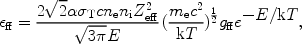(29)

where is the fine structure constant, _T the Thomson cross section, n_e and n_i the electron and ion density, and E the energy of the emitted photon. The factor g_ff is the so-called Gaunt factor and is a dimensionless quantity of order unity. Further, Z_eff is the effective charge of the ion, defined as

(30)

where E_H is the ionisation energy of hydrogen (13.6 eV), I_r the ionisation potential of the ion after a recombination, and n_r the corresponding principal quantum number.

It is also possible to write (29) as _ff = P_ff n_e n_i with

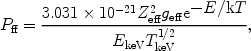(31)

where in this case P_ff is in photons × m³s^-1 keV^-1 and E_keV is the energy in keV. The total amount of radiation produced by this process is given by

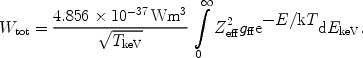(32)

From (29) we see immediately that the Bremsstrahlung spectrum (expressed in W m^-3 keV^-1) is flat for E << kT, and for E > kT it drops exponentially. In order to measure the temperature of a hot plasma, one needs to measure near E kT. The Gaunt factor g_ff can be calculated analytically; there are both tables and asymptotic approximations available. In general, g_ff depends on both E / kT and kT / Z_eff.

For a plasma (29) needs to be summed over all ions that are present in order to calculate the total amount of Bremsstrahlung radiation. For cosmic abundances, hydrogen and helium usually yield the largest contribution. Frequently, one defines an average Gaunt factor G_ff by

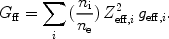(33)

5.1.2. Free-bound emission

Free-bound emission occurs during radiative recombination (Sect. 3.3.1). The energy of the emitted photon is at least the ionisation energy of the recombined ion (for recombination to the ground level) or the ionisation energy that corresponds to the excited state (for recombination to higher levels). From the recombination rate (see Sect. 3.3.1) the free-bound emission is determined immediately:

(34)

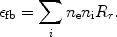
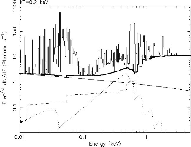
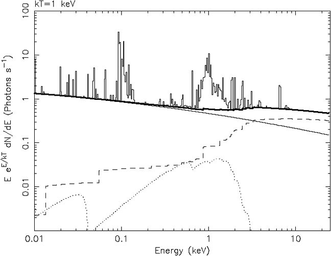
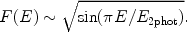
Also here it is possible to define an effective Gaunt factor G_fb. Free-bound emission is in practice often very important. For example in CIE for kT = 0.1 keV, free-bound emission is the dominant continuum mechanism for E > 0.1 keV; for kT = 1 keV it dominates above 3 keV. For kT >> 1 keV Bremsstrahlung is always the most important mechanism, and for kT << 0.1 keV free-bound emission dominates. See also Fig. 8.

Figure 8. Emission spectra of plasmas with solar abundances. The histogram indicates the total spectrum, including line radiation. The spectrum has been binned in order to show better the relative importance of line radiation. The thick solid line is the total continuum emission, the thin solid line the contribution due to Bremsstrahlung, the dashed line free-bound emission and the dotted line two-photon emission. Note the scaling with EeE/kT along the y-axis.

5.1.3. Two photon emission

This process is in particular important for hydrogen-like or helium-like ions. After a collision with a free electron, an electron from a bound 1s shell is excited to the 2s shell. The quantum-mechanical selection rules do not allow that the 2s electron decays back to the 1s orbit by a radiative transition. Usually the ion will then be excited to a higher level by another collision, for example from 2s to 2p, and then it can decay radiatively back to the ground state (1s). However, if the density is very low (n_e << n_{e, crit}, Eqn. 36 - 37), the probability for a second collision is very small and in that case two-photon emission can occur: the electron decays from the 2s orbit to the 1s orbit while emitting two photons. Energy conservation implies that the total energy of both photons should equal the energy difference between the 2s and 1s level (E_2phot = E_1s - E_2s). From symmetry considerations it is clear that the spectrum must be symmetrical around E = 0.5E_2phot, and further that it should be zero for E = 0 and E = E_2phot. An empirical approximation for the shape of the spectrum is given by:

(35)

An approximation for the critical density below which two photon emission is important can be obtained from a comparison of the radiative and collisional rates from the upper (2s) level, and is given by (Mewe et al., 1986):

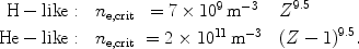(36) (37)

For example for carbon two photon emission is important for densities below 10¹⁷ m^-3, which is the case for many astrophysical applications. Also in this case one can determine an average Gaunt factor G_2phot by averaging over all ions. Two photon emission is important in practice for 0.5 kT 5 keV, and then in particular for the contributions of C, N and O between 0.2 and 0.6 keV. See also Fig. 8.

5.2. Line emission processes

Apart from continuum radiation, line radiation plays an important role for thermal plasmas. In some cases the flux, integrated over a broad energy band, can be completely dominated by line radiation (see Fig. 8). The production process of line radiation can be broken down in two basic steps: the excitation and the emission process.

5.2.1. Excitation process

An atom or ion must first be brought into an excited state before it can emit line photons. There are several physical processes that can contribute to this.

The most important process is usually collisional excitation (Sect. 3.1), in particular for plasmas in CIE. The collision of an electron with the ion brings it in an excited state.

A second way to excite the ion is by absorbing a photon with the proper energy. We discuss this process in more detail in Sect. 6.

Alternatively, inner shell ionisation (either by the collision with a free electron, Sect. 3.2.1 or by the photoelectric effect, Sect. 3.2.2) brings the ion in an excited state.

Finally, the ion can also be brought in an excited state by capturing a free electron in one of the free energy levels above the ground state (radiative recombination, Sect. 3.3.1), or through dielectronic recombination (Sect 3.3.2).

5.2.2. Line emission

It does not matter by whatever process the ion is brought into an excited state j, whenever it is in such a state it may decay back to the ground state or any other lower energy level i by emitting a photon. The probability per unit time that this occurs is given by the spontaneous transition probability A_ij (units: s^-1) which is a number that is different for each transition. The total line power P_ij (photons per unit time and volume) is then given by

(38)

where n_j is the number density of ions in the excited state j. For the most simple case of excitation from the ground state g (rate S_gj) followed by spontaneous emission, one can simply approximate n_g n_eS_gj = n_j A_gj. From this equation, the relative population n_j / n_g << 1 is determined, and then using (38) the line flux is determined. In realistic situations, however, things are more complicated. First, the excited state may also decay to other intermediate states if present, and also excitations or cascades from other levels may play a role. Furthermore, for high densities also collisional excitation or de-excitation to and from other levels becomes important. In general, one has to solve a set of equations for all energy levels of an ion where all relevant population and depopulation processes for that level are taken into account. For the resulting solution vector n_j, the emitted line power is then simply given by Eqn. (38).

Note that not all possible transitions between the different energy levels are allowed. There are strict quantum mechanical selection rules that govern which lines are allowed; see for instance Herzberg (1944) or Mewe (1999). Sometimes there are higher order processes that still allow a forbidden transition to occur, albeit with much smaller transition probabilities A_ij. But if the excited state j has no other (fast enough) way to decay, these forbidden lines occur and the lines can be quite strong, as their line power is essentially governed by the rate at which the ion is brought into its excited state j.

One of the most well known groups of lines is the He-like 1s-2p triplet. Usually the strongest line is the resonance line, an allowed transition. The forbidden line has a similar strength as the resonance line, for the low density conditions in the ISM and intracluster medium, but it can be relatively enhanced in recombining plasmas, or relatively reduced in high density plasmas like stellar coronal loops. In between both lines is the intercombination line. In fact, this intercombination line is a doublet but for the lighter elements both components cannot be resolved. But see Fig. 6 for the case of iron.

5.2.3. Line width

For most X-ray spectral lines, the line profile of a line with energy E can be approximated with a Gaussian exp(-E² / 2²) with given by / E = _v / c where the velocity dispersion is

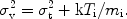(39)

Here T_i is the ion temperature (not necessarily the same as the electron temperature), and _t is the root mean squared turbulent velocity of the emitting medium. For large ion temperature, turbulent velocity or high spectral resolution this line width can be measured, but in most cases the lines are not resolved for CCD type spectra.

5.2.4. Resonance scattering

Resonance scattering is a process where a photon is absorbed by an atom and then re-emitted as a line photon of the same energy into a different direction. As for strong resonance lines (allowed transitions) the transition probabilities A_ij are large, the time interval between absorption and emission is extremely short, and that is the reason why the process effectively can be regarded as a scattering process. We discuss the absorption properties in Sect. 6.3, and have already discussed the spontaneous emission in Sect. 5.2.2.

Resonance scattering of X-ray photons is potentially important in the dense cores of some clusters of galaxies for a few transitions of the most abundant elements, as first shown by Gil'fanov et al. (1987). The optical depth for scattering can be written conveniently as (cf. also Sect. 6.3):

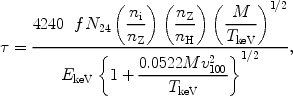(40)

where f is the absorption oscillator strength of the line (of order unity for the strongest spectral lines), E_keV the energy in keV, N₂₄ the hydrogen column density in units of 10²⁴ m^-2, n_i the number density of the ion, n_z the number density of the element, M the atomic weight of the ion, T_keV the ion temperature in keV (assumed to be equal to the electron temperature) and v₁₀₀ the micro-turbulence velocity in units of 100 km/s. Resonance scattering in clusters causes the radial intensity profile on the sky of an emission line to become weaker in the cluster core and stronger in the outskirts, without destroying photons. By comparing the radial line profiles of lines with different optical depth, for instance the 1s-2p and 1s-3p lines of O VII or Fe XXV, one can determine the optical depth and hence constrain the amount of turbulence in the cluster.

Another important application was proposed by Churazov et al. (2001). They show that for WHIM filaments the resonance line of the O VII triplet can be enhanced significantly compared to the thermal emission of the filament due to resonant scattering of X-ray background photons on the filament. The ratio of this resonant line to the other lines of the triplet therefore can be used to estimate the column density of a filament.

5.3. Some important line transitions

In Tables 4 - 5 we list the 100 strongest emission lines under CIE conditions. Note that each line has its peak emissivity at a different temperature. In particular some of the H-like and He-like transitions are strong, and further the so-called Fe-L complex (lines from n = 2 in Li-like to Ne-like iron ions) is prominent. At longer wavelengths, the L-complex of Ne Mg, Si and S gives strong soft X-ray lines. At very short wavelengths, there are not many strong emission lines: between 6-7 keV, the Fe-K emission lines are the strongest spectral features.

Table 4. The strongest emission lines for a plasma with proto-solar abundances (Lodders 2003) in the X-ray band 43 Å < < 100 Å. At longer wavelengths sometimes a few lines from the same multiplet have been added. All lines include unresolved dielectronic satellites. T_max (K) is the temperature at which the emissivity peaks, Q_max = P / (n_e n_H), with P the power per unit volume at T_max, and Q_max is in units of 10^-36 W m³.

E		-log	log	ion	iso-el.	lower	upper
(eV)	(Å)	Qmax	Tmax		seq.	level	level
126.18	98.260	1.35	5.82	Ne VIII	Li	2p 2P3/2	3d 2D5/2
126.37	98.115	1.65	5.82	Ne VIII	Li	2p 2P1/2	3d 2D3/2
127.16	97.502	1.29	5.75	Ne VII	Be	2s 1S0	3p 1P1
128.57	96.437	1.61	5.47	Si V	Ne	2p 1S0	3d 1P1
129.85	95.483	1.14	5.73	Mg VI	N	2p 4S3/2	3d 4P5/2,3/2,1/2
132.01	93.923	1.46	6.80	Fe XVIII	F	2s 2P3/2	2p 2S1/2
140.68	88.130	1.21	5.75	Ne VII	Be	2p 3P1	4d 3D2,3
140.74	88.092	1.40	5.82	Ne VIII	Li	2s 2S1/2	3p 2P3/2
147.67	83.959	0.98	5.86	Mg VII	C	2p 3P	3d 3D, 1D, 3F
148.01	83.766	1.77	5.86	Mg VII	C	2p 3P2	3d 3P2
148.56	83.457	1.41	5.90	Fe IX	Ar	3p 1S0	4d 3P1
149.15	83.128	1.69	5.69	Si VI	F	2p 2P3/2	(3P)3d 2D5/2
149.38	83.000	1.48	5.74	Mg VI	N	2p4 S3/2	4d4 P5/2,3/2,1/2
150.41	82.430	1.49	5.91	Fe IX	Ar	3p 1S0	4d 1P1
154.02	80.501	1.75	5.70	Si VI	F	2p 2P3/2	(1D)3d 2D5/2
159.23	77.865	1.71	6.02	Fe X	Cl	3p 2P1/2	4d 2D5/2
165.24	75.034	1.29	5.94	Mg VIII	B	2p 2P3/2	3d 2D5/2
165.63	74.854	1.29	5.94	Mg VIII	B	2p 2P1/2	3d 2D3/2
170.63	72.663	1.07	5.76	S VII	Ne	2p 1S0	3s 3P1,2
170.69	72.635	1.61	6.09	Fe XI	S	3p 3P2	4d 3D3
171.46	72.311	1.56	6.00	Mg IX	Be	2p 1P1	3d 1D2
171.80	72.166	1.68	6.08	Fe XI	S	3p 1D2	4d 1F3
172.13	72.030	1.44	6.00	Mg IX	Be	2p 3P2,1	3s 3S1
172.14	72.027	1.40	5.76	S VII	Ne	2p 1S0	3s 1P1
177.07	70.020	1.18	5.84	Si VII	O	2p 3P	3d 3D, 3P
177.98	69.660	1.36	6.34	Fe XV	Mg	3p 1P1	4s 1S0
177.99	69.658	1.57	5.96	Si VIII	N	2p 4S3/2	3s 4P5/2,3/2,1/2
179.17	69.200	1.61	5.71	Si VI	F	2p 2P	4d 2P, 2D
186.93	66.326	1.72	6.46	Fe XVI	Na	3d 2D	4f 2F
194.58	63.719	1.70	6.45	Fe XVI	Na	3p 2P3/2	4s 2S1/2
195.89	63.294	1.64	6.08	Mg X	Li	2p 2P3/2	3d 2D5/2
197.57	62.755	1.46	6.00	Mg IX	Be	2s 1S0	3p 1P1
197.75	62.699	1.21	6.22	Fe XIII	Si	3p 3P1	4d 3D2
198.84	62.354	1.17	6.22	Fe XIII	Si	3p 3P0	4d 3D1
199.65	62.100	1.46	6.22	Fe XIII	Si	3p 3P1	4d 3P0
200.49	61.841	1.29	6.07	Si IX	C	2p 3P2	3s 3P1
203.09	61.050	1.06	5.96	Si VIII	N	2p 4S3/2	3d 4P5/2,3/2,1/2
203.90	60.807	1.69	5.79	S VII	Ne	2p 1S0	3d 3D1
204.56	60.610	1.30	5.79	S VII	Ne	2p 1S0	3d 1P1
223.98	55.356	1.00	6.08	Si IX	C	2p 3P	3d 3D, 1D, 3F
234.33	52.911	1.34	6.34	Fe XV	Mg	3s 1S0	4p 1P1
237.06	52.300	1.61	6.22	Si XI	Be	2p 1P1	3s 1S0
238.43	52.000	1.44	5.97	Si VIII	N	2p 4S3/2	4d 4P5/2,3/2,1/2
244.59	50.690	1.30	6.16	Si X	B	2p 2P3/2	3d 2D5/2
245.37	50.530	1.30	6.16	Si X	B	2p 2P1/2	3d 2D3/2
251.90	49.220	1.45	6.22	Si XI	Be	2p 1P1	3d 1D2
252.10	49.180	1.64	5.97	Ar IX	Ne	2p 1S0	3s 3P1,2
261.02	47.500	1.47	6.06	S IX	O	2p 3P	3d 3D, 3P
280.73	44.165	1.60	6.30	Si XII	Li	2p 2P3/2	3d 2D5/2
283.46	43.740	1.46	6.22	Si XI	Be	2s 1S0	3p 1P1

Table 5. As Table 4, but for < 43 Å.

E		-log	log	ion	iso-el.	lower	upper
(eV)	(Å)	Qmax	Tmax		seq.	level	level
291.52	42.530	1.32	6.18	S X	N	2p 4S3/2	3d 4P5/2,3/2,1/2
298.97	41.470	1.31	5.97	C V	He	1s 1S0	2s 3S1 (f)
303.07	40.910	1.75	6.29	Si XII	Li	2s 2S1/2	3p 2P3/2
307.88	40.270	1.27	5.98	C V	He	1s 1S0	2p 1P1 (r)
315.48	39.300	1.37	6.28	S XI	C	2p 3P	3d 3D, 1D, 3F
336.00	36.900	1.58	6.19	S X	N	2p 4S3/2	4d 4P5/2,3/2,1/2
339.10	36.563	1.56	6.34	S XII	B	2p 2P3/2	3d 2D5/2
340.63	36.398	1.56	6.34	S XII	B	2p 2P1/2	3d 2D3/2
367.47	33.740	1.47	6.13	C VI	H	1s 2S1/2	2p 2P1/2 (Ly)
367.53	33.734	1.18	6.13	C VI	H	1s 2S1/2	2p 2P3/2 (Ly)
430.65	28.790	1.69	6.17	N VI	He	1s 1S0	2p 1P1 (r)
500.36	24.779	1.68	6.32	N VII	H	1s 2S1/2	2p 2P3/2 (Ly)
560.98	22.101	0.86	6.32	O VII	He	1s 1S0	2s 3S1 (f)
568.55	21.807	1.45	6.32	O VII	He	1s 1S0	2p 3P2,1 (i)
573.95	21.602	0.71	6.33	O VII	He	1s 1S0	2p 1P1 (r)
653.49	18.973	1.05	6.49	O VIII	H	1s 2S1/2	2p 2P1/2 (Ly)
653.68	18.967	0.77	6.48	O VIII	H	1s 2S1/2	2p 2P3/2 (Ly)
665.62	18.627	1.58	6.34	O VII	He	1s 1S0	3p 1P1
725.05	17.100	0.87	6.73	Fe XVII	Ne	2p 1S0	3s 3P2
726.97	17.055	0.79	6.73	Fe XVII	Ne	2p 1S0	3s 3P1
738.88	16.780	0.87	6.73	Fe XVII	Ne	2p 1S0	3s 1P1
771.14	16.078	1.37	6.84	Fe XVIII	F	2p 2P3/2	3s 4P5/2
774.61	16.006	1.55	6.50	O VIII	H	1s 2S1/2	3p 2P1/2,3/2 (Ly )
812.21	15.265	1.12	6.74	Fe XVII	Ne	2p 1S0	3d 3D1
825.79	15.014	0.58	6.74	Fe XVII	Ne	2p 1S0	3d 1P1
862.32	14.378	1.69	6.84	Fe XVIII	F	2p 2P3/2	3d 2D5/2
872.39	14.212	1.54	6.84	Fe XVIII	F	2p 2P3/2	3d 2S1/2
872.88	14.204	1.26	6.84	Fe XVIII	F	2p 2P3/2	3d 2D5/2
896.75	13.826	1.66	6.76	Fe XVII	Ne	2s 1S0	3p 1P1
904.99	13.700	1.61	6.59	Ne IX	He	1s 1S0	2s 3S1 (f)
905.08	13.699	1.61	6.59	Ne IX	He	1s 1S0	2s 3S1 (f)
916.98	13.521	1.35	6.91	Fe XIX	O	2p 3P2	3d 3D3
917.93	13.507	1.68	6.91	Fe XIX	O	2p 3P2	3d 3P2
922.02	13.447	1.44	6.59	Ne IX	He	1s 1S0	2p 1P1 (r)
965.08	12.847	1.51	6.98	Fe XX	N	2p 4S3/2	3d 4P5/2
966.59	12.827	1.44	6.98	Fe XX	N	2p 4S3/2	3d 4P3/2
1009.2	12.286	1.12	7.04	Fe XXI	C	2p 3P0	3d 3D1
1011.0	12.264	1.46	6.73	Fe XVII	Ne	2p 1S0	4d 3D1
1021.5	12.137	1.77	6.77	Ne X	H	1s 2S1/2	2p 2P1/2 (Ly)
1022.0	12.132	1.49	6.76	Ne X	H	1s 2S1/2	2p 2P3/2 (Ly)
1022.6	12.124	1.39	6.73	Fe XVII	Ne	2p 1S0	4d 1P1
1053.4	11.770	1.38	7.10	Fe XXII	B	2p 2P1/2	3d 2D3/2
1056.0	11.741	1.51	7.18	Fe XXIII	Be	2p 1P1	3d 1D2
1102.0	11.251	1.73	6.74	Fe XVII	Ne	2p 1S0	5d 3D1
1352.1	9.170	1.66	6.81	Mg XI	He	1s 1S0	2p 1P1 (r)
1472.7	8.419	1.76	7.00	Mg XII	H	1s 2S1/2	2p 2P3/2 (Ly)
1864.9	6.648	1.59	7.01	Si XIII	He	1s 1S0	2p 1P1 (r)
2005.9	6.181	1.72	7.21	Si XIV	H	1s 2S1/2	2p 2P3/2 (Ly)
6698.6	1.851	1.43	7.84	Fe XXV	He	1s 1S0	2p 1P1 (r)
6973.1	1.778	1.66	8.17	Fe XXVI	H	1s 2S1/2	2p 2P3/2 (Ly)