


3.1. Initial density perturbation field and its linear evolution
In the currently standard hierarchical structure formation scenario,
objects are thought to form via gravitational collapse of peaks in the
initial primordial density field characterized by the density contrast
(or overdensity) field:
 (x) =
(
(x) =
( (x) -
(x) -
 m) /
m, where
m is the mean mass density of the Universe.
Properties of the field
(x) depend on
specific details
of the processes occurring during the earliest inflationary stage of
evolution of the Universe
(Guth & Pi
1982,
Starobinsky
1982,
Bardeen,
Steinhardt & Turner 1983)
and the subsequent stages prior to recombination
(Peebles 1982,
Bond
& Efstathiou 1984,
Bardeen et
al. 1986,
Eisenstein
& Hu 1999).
A fiducial assumption of most models that we discuss is that
(x) is a
homogeneous and isotropic Gaussian random
field. We briefly discuss non-Gaussian models in
Section 5.1.
m) /
m, where
m is the mean mass density of the Universe.
Properties of the field
(x) depend on
specific details
of the processes occurring during the earliest inflationary stage of
evolution of the Universe
(Guth & Pi
1982,
Starobinsky
1982,
Bardeen,
Steinhardt & Turner 1983)
and the subsequent stages prior to recombination
(Peebles 1982,
Bond
& Efstathiou 1984,
Bardeen et
al. 1986,
Eisenstein
& Hu 1999).
A fiducial assumption of most models that we discuss is that
(x) is a
homogeneous and isotropic Gaussian random
field. We briefly discuss non-Gaussian models in
Section 5.1.
Statistical properties of a uniform and isotropic Gaussian field can
be fully characterized by its power spectrum, P(k), which
depends only on the modulus k of the wavevector, but not on its
direction. A related quantity is the variance of the density contrast field
smoothed on some scale R:
R(x)

 (x -
r)W(r, R)
d3r, where
(x -
r)W(r, R)
d3r, where
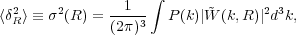 |
(1) |
where
 (k,
R) is the Fourier transform of the window
(filter) function W(r, R), such that
R(k) =
(k)
(k,
R) [see, e.g.,
Zentner 2007
or
Mo, van den Bosch
& White 2010
for details on the definition of
P(k) and choices of window function]. For the cases, when
one is interested in only a narrow range of k the power spectrum
can be approximated by the power-law form, P(k)
(k,
R) is the Fourier transform of the window
(filter) function W(r, R), such that
R(k) =
(k)
(k,
R) [see, e.g.,
Zentner 2007
or
Mo, van den Bosch
& White 2010
for details on the definition of
P(k) and choices of window function]. For the cases, when
one is interested in only a narrow range of k the power spectrum
can be approximated by the power-law form, P(k)
 kn,
and the variance is
kn,
and the variance is
 2(R)
R-(n+3).
2(R)
R-(n+3).
At a sufficiently high redshift z, for the spherical top-hat window
function mass and radius are interchangeable according to the relation
M = 4 /
3m(z)R3. We can think
about the density field smoothed on the scale R or the
corresponding mass scale M. The characteristic amplitude of peaks
in the R (or
m)
field smoothed on scale R (or mass scale M) is given by
(R)
(M). The smoothed
Gaussian density field is, of course, also Gaussian with the probability
distribution function (PDF) given by
/
3m(z)R3. We can think
about the density field smoothed on the scale R or the
corresponding mass scale M. The characteristic amplitude of peaks
in the R (or
m)
field smoothed on scale R (or mass scale M) is given by
(R)
(M). The smoothed
Gaussian density field is, of course, also Gaussian with the probability
distribution function (PDF) given by
 |
(2) |
During the earliest linear stages of evolution in the standard
structure formation scenario the initial Gaussianity of the
(x) field is
preserved, as different Fourier modes
(k) evolve
independently and grow
at the same rate, described by the linear growth factor,
D+(a), as a function of expansion factor
a = (1 + z)-1, which for a
 CDM cosmology is
given by
Heath (1977):
CDM cosmology is
given by
Heath (1977):
 |
(3) |
where E(a) is the normalized expansion rate, which is given by
 |
(4) |
if the contribution from relativistic species, such as radiation or neutrinos, to the energy-density is neglected. Growth rate and the expression for E(a) in more general, homogeneous dark energy (DE) cosmologies are described by Percival (2005). Note that in models in which DE is clustered (Alimi et al. 2010) or gravity deviates from General Relativity (GR, see Section 5.2), the growth factor can be scale dependent.
Correspondingly, the linear evolution of the root mean square (rms)
amplitude of fluctuations is given by
(M, a) =
(M,
ai)D+(a)
/ D+(ai), which is often useful to
recast in terms of linearly extrapolated rms amplitude
(M, a = 1)
at a = 1 (i.e., z = 0):
 |
(5) |
Once the amplitude of typical fluctuations approaches unity,
(M, a) ~
1, the linear approximation breaks
down. Further evolution must be studied by means of nonlinear models or
direct numerical simulations. We discuss results of numerical
simulations extensively below. However, we consider first the
simplified, but instructive, spherical collapse model and associated
concepts and terminology. Such model can be used to gain physical
insight into the key features of the evolution and is used as a basis
for both definitions of collapsed objects (see
Section 3.6) and quantitative models for halo abundance
and clustering (Section 3.7 and 3.8).
3.2. Non-linear evolution of spherical perturbations and non-linear mass scale
The simplest model of non-linear collapse assumes that density peak can be characterized as constant overdensity spherical perturbation of radius R. Despite its simplicity and limitations discussed below, the model provides a useful insight into general features and timing of non-linear collapse. Its results are commonly used in analytic models for halo abundance and clustering and motivate mass definitions for collapsed objects. Below we briefly describe the model and non-linear mass scale that is based on its predictions.
3.2.1. Spherical collapse model
The spherical collapse model considers a
spherically-symmetric density fluctuation of initial radius
Ri, amplitude
i > 0, and
mass
M = (4/3)(1 +
i)
Ri3, where
Ri is physical radius of the perturbation and
is
the mean density of the Universe at the initial time. Given the
symmetry, the collapse of such perturbation is a one-dimensional
problem and is fully specified by evolution of the top-hat radius
R(t)
(Gunn &
Gott 1972,
Lahav et
al. 1991).
It consists of an initially decelerating increase of the perturbation
radius, until it reaches the maximum value, Rta, at
the turnaround epoch,
tta, and subsequent decrease of R(t) at
t > tta
until the perturbation collapses, virializes, and settles at the final
radius Rf at t =
tcoll. Physically, Rf is
set by the virial relation between potential and kinetic energy and is
Rf = Rta / 2 in cosmologies with
 =
0. The turnaround epoch and the epoch of collapse and virialization are
defined by initial conditions.
=
0. The turnaround epoch and the epoch of collapse and virialization are
defined by initial conditions.
The final mean internal density of a collapsed object can be estimated
by noting that in a = 0 Universe the time
interval tcoll - tta =
tta should be equal to the free-fall time
of a uniform sphere tff =
[3 / (32G
ta]1/2, which
means that the mean density of perturbation at turnaround is
ta =
3 /
(32Gtta2) and
coll
= 8ta = 3 /
(Gtcoll2). These densities can be compared
with background mean matter densities at the corresponding times to get
mean internal density contrasts:
 =
/ m. In the Einstein-de Sitter model
(m = 1,
=
0), background density evolves as
m = 1 /
(6 G
t2), which means that density contrast
after virialization is
=
/ m. In the Einstein-de Sitter model
(m = 1,
=
0), background density evolves as
m = 1 /
(6 G
t2), which means that density contrast
after virialization is
 |
(6) |
For general cosmologies, density contrast can be computed by
estimating
coll
and
m(tcoll) in a
similar fashion. For lower
m models,
fluctuation of the same mass
M and has a
larger initial radius and smaller physical
density and, thus, takes longer to collapse. The density contrasts of
collapsed objects therefore are larger in lower density models because
the mean density of matter at the time of collapse is
smaller. Accurate (to
 1% for
m = 0.1 -
1) approximations
for vir
in open
( =
0) and flat
CDM
(1 - -
m = 0)
cosmologies are given by Bryan & Norman
(1998,
their equation 6). For example, for the concordance
CDM
cosmology with
m = 0.27 and
= 0.73
(Komatsu et
al. 2011),
density contrast at z = 0 is
vir
1% for
m = 0.1 -
1) approximations
for vir
in open
( =
0) and flat
CDM
(1 - -
m = 0)
cosmologies are given by Bryan & Norman
(1998,
their equation 6). For example, for the concordance
CDM
cosmology with
m = 0.27 and
= 0.73
(Komatsu et
al. 2011),
density contrast at z = 0 is
vir
 358.
358.
Note that if the initial density contrast
i would grow
only at the linear rate, D+(z), then the
density contrast at the time of
collapse would be more than a hundred times smaller. Its value can be
derived starting from the density contrast linearly extrapolated to
the turn around epoch,
ta. This
epoch corresponds to
the time at which perturbation enters in the non-linear regime and
detaches from the Hubble expansion, so that
ta ~ 1
is expected. In fact, the exact calculation in the case of
m(z) = 1 at the redshift of turn-around
gives ta = 1.062
(Gunn &
Gott 1972).
Because tcoll = 2tta, further linear
evolution for
m(z)
= 1 until the collapse time gives
c =
ta
D+(tc)
/ D+(tta)
1.686. In the
case of m
 1 we expect that
ta should have
different values. For instance, for
m < 1
density contrast at
turn-around should be higher to account for the higher rate of the
Hubble expansion. However, linear growth from
tta to tcoll is smaller due to the
slower redshift dependence of
D+(z). As a matter of fact, these two factors
nearly cancel, so that
c has a weak
dependence on
m and
(e.g.,
Percival 2005).
For the concordance
CDM cosmology at
z = 0, for example,
c
1.675.
1 we expect that
ta should have
different values. For instance, for
m < 1
density contrast at
turn-around should be higher to account for the higher rate of the
Hubble expansion. However, linear growth from
tta to tcoll is smaller due to the
slower redshift dependence of
D+(z). As a matter of fact, these two factors
nearly cancel, so that
c has a weak
dependence on
m and
(e.g.,
Percival 2005).
For the concordance
CDM cosmology at
z = 0, for example,
c
1.675.
Additional interesting effects may arise in models with DE characterized by small or zero speed of sound, in which structure growth is affected not only because DE influences linear growth, but also because it participates non-trivially in the collapse of matter and may slow down or accelerate the formation of clusters of a given mass depending on DE equation of state (Abramo et al. 2007, Creminelli et al. 2010). DE in such models can also contribute non-trivially to the gravitating mass of clusters.
3.2.2. The nonlinear mass scale MNL
The linear value of the collapse overdensity
c is useful in
predicting whether a given initial perturbation
i ≪ 1 at
initial zi collapses by some later redshift
z. The collapse condition is simply
i
D+0(z)
 c(z)
and is used extensively to model the abundance and clustering of collapsed
objects, as we discuss below in Section 3.7. The
distribution of
peak amplitudes in the initial Gaussian overdensity field smoothed
over mass scale M is given by a Gaussian PDF with a rms value of
(M) (Equation
2). The peaks in the initial
Gaussian overdensity field smoothed at redshift zi
over mass scale M can be characterized by the ratio
c(z)
and is used extensively to model the abundance and clustering of collapsed
objects, as we discuss below in Section 3.7. The
distribution of
peak amplitudes in the initial Gaussian overdensity field smoothed
over mass scale M is given by a Gaussian PDF with a rms value of
(M) (Equation
2). The peaks in the initial
Gaussian overdensity field smoothed at redshift zi
over mass scale M can be characterized by the ratio
 =
i /
(M,
zi)
called the peak height. For a given mass scale M, the peaks
collapsing at a given redshift z according to the spherical collapse
model have the peak height given by:
=
i /
(M,
zi)
called the peak height. For a given mass scale M, the peaks
collapsing at a given redshift z according to the spherical collapse
model have the peak height given by:
 |
(7) |
Given that
c(z)
is a very weak function of z (changing by
1-2% typically),
whereas
(M, z) =
(M, z =
0)D+0(z) decreases
strongly with increasing z, the peak height of collapsing objects
of a given mass M increases rapidly with increasing redshift.
Using Equation 7 we can define the characteristic mass scale for
which a typical peak ( = 1)
collapses at redshift z:
 |
(8) |
This nonlinear mass, MNL(z), is a key quantity in the self-similar models of structure formation, which we consider in Section 3.9.
3.3. Nonlinear collapse of real density peaks
The spherical collapse model provides a useful approximate guideline for the time scale of halo collapse and has proven to be a very useful tool in developing approximate statistical models for the formation and evolution of halo populations. Such a simple model and its extensions (e.g., ellipsoidal collapse model) do, however, miss many important details and complexities of collapse of the real density peaks. Such complexities are usually explored using three-dimensional numerical cosmological simulations. Techniques and numerical details of such simulations are outside the scope of this review and we refer readers to recent reviews on this subject (Bertschinger 1998, Dolag et al. 2008, Norman 2010, Borgani & Kravtsov 2011). Here, we simply discuss the main features of gravitational collapse learned from analyses of such simulations.
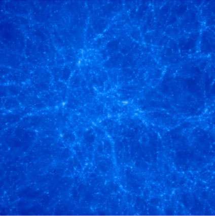
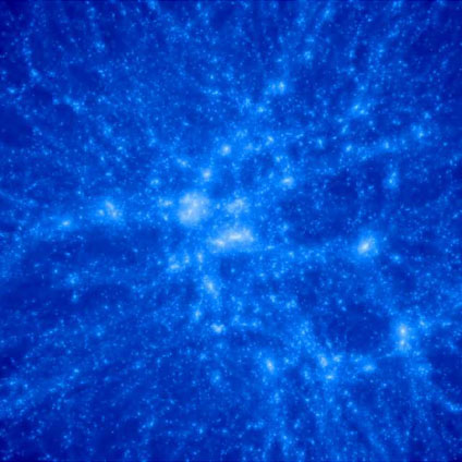
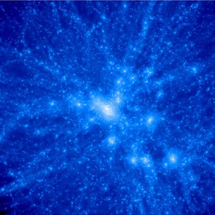
Figure 6 shows evolution of the DM density field in a cosmological simulation of a comoving region of 15h-1 Mpc on a side around cluster mass-scale density peak in the initial perturbation field from z = 3 to the present epoch. The overall picture is quite different from the top-hat collapse. First of all, real peaks in the primordial field do not have the constant density or sharp boundary of the top-hat, but have a certain radial profile and curvature (Bardeen et al. 1986, Dalal et al. 2008). As a result, different regions of a peak collapse at different times so that the overall collapse is extended in time and the peak does not have a single collapse epoch (e.g., Diemand, Kuhlen & Madau 2007). Consequently, the distribution of matter around the collapsed peak can smoothly extend to several virial radii for late epochs and small masses (Prada et al. 2006, Cuesta et al. 2008). This creates ambiguity about the definition of halo mass and results in a variety of mass definitions adopted in practice, as we discuss in Section 3.6.
 |
 |
 |
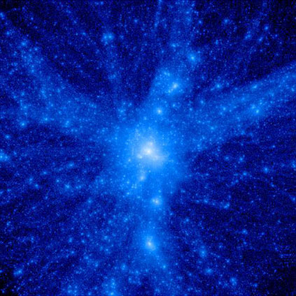 |
Figure 6. Evolution of a dark matter
density field in a comoving region of 15h-1 Mpc on a
side around cluster mass density peak in the
initial perturbation field. The four panels, from top left to
bottom right, show redshifts z = 3, z = 1, z = 0.5
and z = 0. The forming cluster has a mass M200
|
|
Second, the peaks in the smoothed density field,
R(x),
are not isolated but are surrounded by other peaks and density
inhomogeneities. The tidal forces from the most massive and rarest
peaks in the initial density field shepherd the surrounding matter
into massive filamentary structures that connect them
(Bond, Kofman
& Pogosyan 1996).
Accretion of matter onto clusters at late epochs occurs
preferentially along such filaments, as can be clearly seen in
Figure 6.
Finally, the density distribution within the peaks in the actual
density field is not smooth, as in the smoothed field
R(x),
but contains fluctuations on all scales. Collapse of
density peaks on different scales can proceed almost simultaneously,
especially during early stages of evolution in the CDM models when
peaks undergoing collapse involve small scales, over which the power
spectrum has an effective slope n
-3.
Figure 6
shows that at high redshifts the proto-cluster region contains mostly
small-mass collapsed objects, which merge to form a larger and larger
virialized system near the center of the shown region at later
epochs. Nonlinear interactions between smaller-scale peaks within a
cluster-scale peak during mergers result in relaxation processes and
energy exchange on different scales, and mass redistribution. Although
the processes accompanying major mergers are not as violent as
envisioned in the violent relaxation scenario
(Valluri et
al. 2007),
such interactions lead to significant redistribution of mass
(Kazantzidis, Zentner & Kravtsov 2006)
and angular momentum
(Vitvitska
et al. 2002),
both within and outside of the virial radius.
Following the collapse, matter settles into an equilibrium
configuration. For collisional baryonic component this configuration
is approximately described by the hydrostatic equilibrium (HE
hereafter) equation, in which the pressure gradient
 p(x) at
point x is balanced by the gradient of local gravitational
potential
p(x) at
point x is balanced by the gradient of local gravitational
potential  (x):
(x) =
-
p(x) /
g(x), where
g(x) is the gas
density. Under the further assumption of spherical symmetry, the HE
equation can be written as
g-1dp /
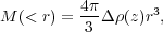
dr = -GM(< r) / r2, where
M(< r) is the mass contained within the radius
r. Assuming the equation of state of ideal gas, p
= g
kB T /
µ mp where
µ is the mean molecular weight and mp is the
proton mass; cluster mass within r can be expressed in terms of
the density and temperature profiles,
g(r) and T(r), as
(x):
(x) =
-
p(x) /
g(x), where
g(x) is the gas
density. Under the further assumption of spherical symmetry, the HE
equation can be written as
g-1dp /
dr = -GM(< r) / r2, where
M(< r) is the mass contained within the radius
r. Assuming the equation of state of ideal gas, p
= g
kB T /
µ mp where
µ is the mean molecular weight and mp is the
proton mass; cluster mass within r can be expressed in terms of
the density and temperature profiles,
g(r) and T(r), as
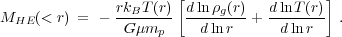 |
(9) |
Interestingly, the slopes of the gas density and temperature profiles that enter the above equation exhibit correlation that appears to be a dynamical attractor during cluster formation (Juncher, Hansen & Macciò 2012).
For a collisionless system of particles, such as CDM, the condition of equilibrium is given by the Jeans equation (e.g., Binney & Tremaine 2008). For a non-rotating spherically symmetric system, this equation can be written as
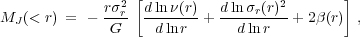 |
(10) |
where  = 1 -
t2 /
2r2
is the orbit anisotropy
parameter defined in terms of the radial
(r) and
tangential
(t) velocity
dispersion components
( = 0 for
isotropic velocity field). We consider equilibrium density and velocity
dispersion profiles, as well as anisotropy profile
(r) in
Section 3.5.2. Equation 10 is also commonly used
to describe the equilibrium of cluster galaxies. Although, in
principle, galaxies in groups and clusters are not strictly
collisionless, interactions between galaxies are relatively rare and
the Jeans equation should be quite accurate.
= 1 -
t2 /
2r2
is the orbit anisotropy
parameter defined in terms of the radial
(r) and
tangential
(t) velocity
dispersion components
( = 0 for
isotropic velocity field). We consider equilibrium density and velocity
dispersion profiles, as well as anisotropy profile
(r) in
Section 3.5.2. Equation 10 is also commonly used
to describe the equilibrium of cluster galaxies. Although, in
principle, galaxies in groups and clusters are not strictly
collisionless, interactions between galaxies are relatively rare and
the Jeans equation should be quite accurate.
Note that the difference between equilibrium configuration of collisional ICM and collisionless DM and galaxy systems is significant. In HE, the iso-density surfaces of the ICM should trace the iso-potential surfaces. The shape of the iso-potential surfaces in equilibrium is always more spherical than the shape of the underlying mass distribution that gives rise to the potential. Given that the potential is dominated by DM at most of the cluster-centric radii, the ICM distribution (and consequently the X-ray isophotes and SZ maps) will be more spherical than the underlying DM distribution.
As we noted in the previous section, the gravitational collapse of a
halo is a process extended in time. Consequently, a cluster may not
reach complete equilibrium over the Hubble time due to ongoing
accretion of matter and the occurrence of minor and major mergers. The
ICM reaches equilibrium state following a major merger only after
3-4 Gyr (e.g.,
(Nelson et
al. 2011)).
Deviations from equilibrium affect observable properties of clusters and
cause systematic errors when equations 9 and 10 are used to estimate
cluster masses (e.g.,
Rasia, Tormen
& Moscardini 2004,
Nagai,
Kravtsov & Vikhlinin 2007,
Ameglio et
al. 2009,
Piffaretti
& Valdarnini 2008,
Lau, Kravtsov
& Nagai 2009).
3.5. Internal structure of cluster halos
Relaxations processes establish the equilibrium internal structure of clusters. Below we review our current undertstanding of the equilibrium radial density distribution, velocity dispersion, and triaxiality (shape) of the cluster DM halos.
Internal structure of collapsed halos may be expected to depend both on the properties of the initial density distribution around collapsing peaks (Hoffman & Shaham 1985) and on the processes accompanying hierarchical collapse (e.g., Syer & White 1998, Valluri et al. 2007). The fact that simulations have demonstrated that the characteristic form of the spherically averaged density profile arising in CDM models, characterized by the logarithmic slope steepening with increasing radius (Dubinski & Carlberg 1991, Katz 1991, Navarro, Frenk & White 1995, 1996), is virtually independent of the shape of power spectrum and background cosmology (Katz 1991, Cole & Lacey 1996, Navarro, Frenk & White 1997, Huss, Jain & Steinmetz 1999b) is non trivial. Such a generic form of the profile also arises when small-scale structure is suppressed and the collapse is smooth, as is the case for halos forming at the cut-off scale of the power spectrum (Moore et al. 1999, Diemand, Moore & Stadel 2005, Wang & White 2009) or even from non-cosmological initial conditions (Huss, Jain & Steinmetz 1999a).
The density profiles measured in dissipationless simulations are most commonly approximated by the "NFW" form proposed by (Navarro, Frenk & White 1995) based on their simulation of cluster formation:
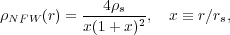 |
(11) |
where rs is the scale radius, at which the logarithmic
slope of the profile is equal to -2 and
s
is the characteristic density at
r = rs. Overall, the slope of this profile
varies with radius as
dln /
dlnr = -[1 + 2x / (1 + x)], i.e., from the
asymptotic slope of
-1 at x ≪ 1 to -3 at x ≫ 1, where the enclosed
mass diverges logarithmically: M(< r) =
M
f(x) / f(c), where
M
is the mass enclosing a given overdensity
,
f(x)
ln(1 + x) -
x / (1 + x) and
c
R /
rs is
the concentration parameter. Accurate formulae for the conversion of
mass of the NFW halos defined for different values of
are given
in the appendix of
(Hu &
Kravtsov 2003).
Subsequent simulations (Navarro et al. 2004, Merritt et al. 2006, Graham et al. 2006) showed that the Einasto (1965) profile and other similar models designed to describe de-projection of the Sérsic profile (Merritt et al. 2006) provide a more accurate description of the DM density profiles arising during cosmological halo collapse, as well as profiles of bulges and elliptical galaxies (Cardone, Piedipalumbo & Tortora 2005). The Einasto profile is characterized by the logarithmic slope that varies as a power law with radius:
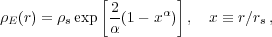 |
(12) |
where rs is again the scale radius at which the
logarithmic slope is -2, but now for the Einasto profile,
s
e(rs), and
 is an additional
parameter that describes the power-law dependence of the logarithmic
slope on radius:
dlne / dlnr =
-2x.
is an additional
parameter that describes the power-law dependence of the logarithmic
slope on radius:
dlne / dlnr =
-2x.
Note that unlike the NFW profile and several other profiles discussed
in the literature, the Einasto profile does not have an asymptotic
slope at small radii. The slope of the density profile becomes
increasingly shallower at small radii at the rate controlled by
. The parameter
varies with halo mass
and redshift: at z = 0 galaxy-sized halos are described by
0.16,
whereas massive cluster halos are described by
0.2-0.3; these values increase by ~ 0.1 by z
3
(Gao et
al. 2008).
Although depends on
mass and redshift (and thus also on the cosmology) in a non-trivial way,
(Gao et
al. 2008],
and see also
Duffy et
al. 2008)
showed that these dependencies can be captured as a universal
dependence on the peak height
=
c /
(M, z) (see
Section 3.2.2 above):
=
0.00952 +
0.155. Finally,
unlike the NFW profile, the total mass for the Einasto profile is
finite due to the exponentially decreasing density at large radii. A
number of useful expressions for the Einasto profile, such as mass
within a radius, are provided by
Cardone,
Piedipalumbo & Tortora (2005),
Mamon &
okas (2005),
and
Graham et
al. (2006).
The origin of the generic form of the density profile has recently
been explored in detail by
Lithwick
& Dalal (2011),
who show that it
arises due to two main factors: (a) the density and triaxiality
profile of the original peak and (b) approximately adiabatic
contraction of the previously collapsed matter due to deepening of the
potential well during continuing collapse. Without adiabatic
contraction the profile resulting from the collapse would reflect the
shape of the initial profile of the peak. For example, if the initial
profile of mean linear overdensity within radius r around the peak
can be described as
 L
rL-
L
rL- ,
it can be shown that the resulting differential density profile after
collapse without adiabatic contraction behaves as
(r)
r-g, where g =
3 / (1 +
)
(Fillmore
& Goldreich 1984).
Typical profiles of
initial density peaks are characterized by shallow slopes,
~
0-0.3 at small radii, and very steep slopes at large radii (e.g.,
Dalal et
al. 2008),
which means that resulting
profiles after collapse should have slopes varying from
g
0-0.7 at small radii to g
3 at large radii.
,
it can be shown that the resulting differential density profile after
collapse without adiabatic contraction behaves as
(r)
r-g, where g =
3 / (1 +
)
(Fillmore
& Goldreich 1984).
Typical profiles of
initial density peaks are characterized by shallow slopes,
~
0-0.3 at small radii, and very steep slopes at large radii (e.g.,
Dalal et
al. 2008),
which means that resulting
profiles after collapse should have slopes varying from
g
0-0.7 at small radii to g
3 at large radii.
However,
Lithwick
& Dalal (2011)
showed that contraction of particle
orbits during subsequent accretion of mass interior to a given radius
r leads to a much more gradual change of logarithmic slope with
radius, such that the regime within which g
0-0.7 is shifted
to very small radii (r / rvir
10-5),
whereas at the radii typically resolved in cosmological simulations the
logarithmic slope is in the range of g
1-3, so that the
radial dependence of the logarithmic slope g(r) =
dln /
dlnr is in good qualitative
agreement with simulation results. This contraction occurs because
matter that is accreted by a halo at a given stage of its evolution
can deposit matter over a wide range of radii, including small
radii. The orbits of particles that accreted previously have to
respond to the additional mass, and they do so by contracting. For
example, for a purely spherical system in which mass is added slowly
so that the adiabatic invariant is conserved, radii r of spherical
shells must decrease to compensate an increase of M(<
r). This model thus elegantly explains both the qualitative shape
of density profiles observed in cosmological simulations and their
universality. The latter can be expected because the contraction process
crucial to shaping the form of the profile should operate under general
collapse conditions, in which different shells of matter collapse at
different times.
Although the model of Lithwick & Dalal (2011) provides a solid physical picture of halo profile formation, it also neglects some of the processes that may affect details of the resulting density profile, most notably the effects of mergers. Indeed, major mergers lead to resonant dynamical heating of a certain fraction of collapsed matter due to the potential fluctuations and tidal forces that they induce. The amount of mass that is affected by such heating is significant (e.g., Valluri et al. 2007). In fact, up to ~ 40% of mass within the virial radii of merging halos may end up outside of the virial radius of the merger. This implies, for example, that virial mass is not additive in major mergers. Nevertheless, in practice the merger remnant retains the functional form of the density profiles of the merger progenitors (Kazantzidis, Zentner & Kravtsov 2006), which means that major mergers do not lead to efficient violent relaxation.
Although the functional form of the density profile arising during
halo collapse is generic for a wide variety of collapse conditions and
models, initial conditions and cosmology do significantly affect
the physical properties of halo profiles
such as its characteristic density and scale radius
(Navarro,
Frenk & White 1997).
These dependencies are often discussed in terms of halo concentrations,
c
R / rs.
Simulations show that the scale radius is approximately constant
during late stages of halo evolution
(Bullock et
al. 2001,
Wechsler et
al. 2002),
but evolves as rs = cmin
R
during early stages, when a halo quickly
increases its mass through accretion and mergers
(Zhao et
al. 2003,
Zhao et
al. 2009).
The minimum value of concentration is cmin = const
3-4 for
= 200. For massive
cluster halos, which are in the fast growth regime at any redshift,
the concentrations are thus expected to stay approximately constant
with redshift or may even increase after reaching a minimum
(Klypin,
Trujillo-Gomez & Primack 2011,
Prada et
al. 2012).
The characteristic time separating the two regimes can be identified
as the formation epoch of halos. This time approximately determines
the value of the scale radius and the subsequent evolution of halo
concentration. The initial conditions and cosmology determine the
formation epoch and the typical mass accretion histories for halos of
a given mass
(Navarro,
Frenk & White 1997,
Bullock et
al. 2001,
Zhao et
al. 2009),
and therefore determine the halo concentrations. Although these
dependences are non-trivial functions of halo mass and redshift, they
can also be encapsulated by a universal function of the peak height
(Zhao et
al. 2009,
Prada et
al. 2012).
Baryon dissipation and feedback are expected to affect the density
profiles of halos appreciably, although predictions for these effects
are far less certain than predictions of the DM distribution in the
purely dissipationless regime. The main effect is contraction of DM in
response to the increasing depth of the central potential during
baryon cooling and condensation, which is often modelled under the
assumption of slow contraction conserving adiabatic invariants of
particle orbits (e.g.,
Zeldovich
et al. 1980,
Barnes &
White 1984,
Blumenthal
et al. 1986,
Ryden &
Gunn 1987).
The standard model of such adiabatic contraction assumes that DM
particles are predominantly on circular orbits, and for each shell of
DM at radius r the product of the radius and the enclosed mass
rM(r) is conserved
(Blumenthal
et al. 1986).
The model makes a
number of simplifying assumptions and does not take into account
effects of mergers. Nevertheless, it was shown to provide a reasonably
accurate description of the results of cosmological simulations
(Gnedin et
al. 2004).
Its accuracy can be further improved by
relaxing the assumption of circular orbits and adopting an empirical
ansäz, in which the conserved quantity is
rM( ), where
is the average radius
along the particle orbit, instead of rM(r)
(Gnedin et
al. 2004).
At the same time, several recent
studies showed that no single set of parameters of such simple models
describes all objects that form in cosmological simulations equally well
(Gustafsson,
Fairbairn & Sommer-Larsen 2006,
Abadi et
al. 2010,
Tissera et
al. 2010,
Gnedin et
al. 2011).
), where
is the average radius
along the particle orbit, instead of rM(r)
(Gnedin et
al. 2004).
At the same time, several recent
studies showed that no single set of parameters of such simple models
describes all objects that form in cosmological simulations equally well
(Gustafsson,
Fairbairn & Sommer-Larsen 2006,
Abadi et
al. 2010,
Tissera et
al. 2010,
Gnedin et
al. 2011).
A more subtle but related effect is the increase of the overall concentration of DM within the virial radius of halos due to re-distribution of binding energy between DM and baryons during the process of cluster assembly (Rudd, Zentner & Kravtsov 2008). The larger range of radii over which this effect operates makes it a potential worry for the precision constraints from the cosmic shear power spectrum (Jing et al. 2006, Rudd, Zentner & Kravtsov 2008). This effect depends primarily on the fraction of baryons that condense into the central halo galaxies and may be mitigated by the blow-out of gas by efficient AGN or SN feedback (van Daalen et al. 2011). The effects of baryons on the overall concentration of mass distribution in clusters are thus uncertain, but can potentially increase halo concentration and thereby significantly enhance the cross section for strong lensing (Puchwein et al. 2005, Rozo et al. 2008, Mead et al. 2010) and affect statistics of strong lens distribution in groups and clusters (e.g., More et al. 2011).
A number of studies have derived observational constraints on density
profiles of clusters and their concentrations
(Pointecouteau, Arnaud & Pratt 2005,
Vikhlinin
et al. 2006,
Schmidt
& Allen 2007,
Buote et
al. 2007,
Mandelbaum,
Seljak & Hirata 2008,
Wojtak &
okas 2010,
Okabe et
al. 2010,
Ettori et
al. 2010,
Umetsu et
al. 2011b,
Umetsu et
al. 2011a,
Sereno
& Zitrin 2012).
Although most of these studies find that the concentrations of galaxy
clusters predicted by
CDM simulations
are in the ballpark of
values derived from observations, the agreement is not perfect and
there is tension between model predictions and observations, which may
be due to effects of baryon dissipation (e.g.,
Rudd, Zentner
& Kravtsov 2008,
Fedeli 2012).
Some studies do find that the concordance cosmology predictions of the average cluster concentrations are somewhat lower than the average values derived from X-ray observations (Schmidt & Allen 2007, Buote et al. 2007, Duffy et al. 2008). Moreover, lensing analyses indicate that the slope of the density profile in central regions of some clusters may be shallower than predicted (Tyson, Kochanski & dell'Antonio 1998, Sand et al. 2004, Sand et al. 2008, Newman et al. 2009, Newman et al. 2011), whereas concentrations are considerably higher than both theoretical predictions and most other observational determinations from X-ray and WL analyses (Comerford & Natarajan 2007, Oguri et al. 2009, Oguri et al. 2012, Zitrin et al. 2011).
At this point, it is not clear whether these discrepancies imply
serious challenges to the
CDM structure
formation paradigm,
unknown baryonic effects flattening the profiles in the centers, or
unaccounted systematics in the observational analyses (e.g.,
Dalal &
Keeton 2003,
Hennawi et
al. 2007).
When considering such
comparisons, it is important to remember that density profiles in
cosmological simulations are always defined with respect to the center
defined as the global density peak or potential minimum, whereas in
observations the corresponding location is not as unambiguous as
in simulations and the choice of center may affect the derived slope.
It should be noted that improved theoretical predictions for
cluster-sized systems generally predict larger concentrations for the
most massive objects than do extrapolations of the concentration-mass
relations from smaller mass objects
(Zhao et
al. 2009,
Prada et
al. 2012,
Bhattacharya, Habib & Heitmann 2011).
In addition, as
we noted above, the evolution predicted for the concentrations of
these rarest objects is much weaker than c
(1 + z) found for
smaller mass halos, so rescaling the concentrations of high-redshift
clusters by (1 + z) factor, as is often done, could lead to an
overestimate of their concentrations.
3.5.2. Velocity dispersion profile and velocity anisotropy
Velocity dispersion profile is a halo property related to its density
profile. Simulations show that this profile generally increases from
the central value to a maximum at r
rs and slowly decreases outward (e.g.,
Cole &
Lacey 1996,
Rasia, Tormen
& Moscardini 2004).
One remarkable result illustrating the close connection between density
and velocity dispersion is that for collapsed halos in dissipationless
simulations the ratio of density to the cube of the rms velocity
dispersion can be accurately described by a power law over at least
three decades in radius
(Taylor
& Navarro 2001):
Q(r)
/
3
r-
with
1.9.
An important quantity underlying the measured velocity dispersion
profile is the profile of the mean velocity, and the mean radial
velocity,
 r,
in particular. For a spherically
symmetric matter distribution in HE, we expect
r =
0. Therefore, the profile of
r is a useful
diagnostic of deviations from equilibrium at different
radii. Simulations show that clusters at z = 0 generally have zero
mean radial velocities within r
Rvir and turn sharply negative between 1 and
3Rvir, where density is
dominated by matter infalling onto cluster
(Cole &
Lacey 1996,
Eke, Navarro
& Frenk 1998,
Cuesta et
al. 2008).
r,
in particular. For a spherically
symmetric matter distribution in HE, we expect
r =
0. Therefore, the profile of
r is a useful
diagnostic of deviations from equilibrium at different
radii. Simulations show that clusters at z = 0 generally have zero
mean radial velocities within r
Rvir and turn sharply negative between 1 and
3Rvir, where density is
dominated by matter infalling onto cluster
(Cole &
Lacey 1996,
Eke, Navarro
& Frenk 1998,
Cuesta et
al. 2008).
The distinguishing characteristic between gas and DM is the fact that
gas has an isotropic velocity dispersion tensor on small scales,
whereas DM in general does not. On large scales, however, both gas and
DM may have velocity fields that are anisotropic. The degree of
velocity anisotropy is commonly quantified by the anisotropy profile,
(r)
(see Section 3.4). DM anisotropy is mild:
0-0.1 near the
center and increases to
0.2-0.4 near the virial radius
(Cole &
Lacey 1996,
Eke, Navarro
& Frenk 1998,
Colín,
Klypin & Kravtsov 2000,
Rasia, Tormen
& Moscardini 2004,
Lemze et
al. 2011).
Interestingly, velocities exhibit substantial tangential anisotropy
outside the virial radius in the infall region of clusters
(Cuesta et
al. 2008,
Lemze et
al. 2011).
Another interesting finding is that the velocity anisotropy correlates
with the slope of the density profile
(Hansen
& Moore 2006),
albeit with significant scatter
(Lemze et
al. 2011).
The gas component also has some residual motions driven by mergers and gas accretion along filaments. Gas velocities tend to have tangential anisotropy (Rasia, Tormen & Moscardini 2004), because radial motions are inhibited by the entropy profile, which is convectively stable in general.
Although the density structure of mass distribution in clusters is most often described by spherically averaged profiles, clusters are thought to collapse from generally triaxial density peaks (Doroshkevich 1970, Bardeen et al. 1986). The distribution of matter within halos resulting from hierarchical collapse is triaxial as well (Frenk et al. 1988, Dubinski & Carlberg 1991, Warren et al. 1992, Cole & Lacey 1996, Jing & Suto 2002, Kasun & Evrard 2005, Allgood et al. 2006), with triaxiality predicted by dissipationless simulations increasing with decreasing distance from halo center (Allgood et al. 2006). Triaxiality of halos decreases with decreasing mass and redshift (Kasun & Evrard 2005, Allgood et al. 2006) in a way that again can be parameterized in a universal form as a function of peak height (Allgood et al. 2006). The major axis of the triaxial distribution of clusters is generally aligned with the filament connecting a cluster with its nearest neighbor of comparable mass (e.g., West & Blakeslee 2000, Lee et al. 2008), which reflects the fact that a significant fraction of mass and mergers is occurring along such filaments (e.g., Onuora & Thomas 2000, Lee & Evrard 2007).
Jing & Suto (2002) showed how the formalism of density distribution as a function of distance from cluster center can be extended to the density distribution in triaxial shells. Accounting for such triaxiality is particularly important in theoretical predictions and observational analyses of weak and strong lensing (Dalal & Keeton 2003, Clowe, De Lucia & King 2004, Oguri et al. 2005, Corless & King 2007, Hennawi et al. 2007, Becker & Kravtsov 2011). At the same time, it is important to keep in mind that, as with many other results derived mainly from dissipationless simulations, the physics of baryons may modify predictions substantially.
The shape of the DM distribution in particular is quite sensitive to the degree of central concentration of mass. As baryons condense towards the center to form a central galaxy within a halo, the DM distribution becomes more spherical (Dubinski 1994, Evrard, Summers & Davis 1994, Tissera & Dominguez-Tenreiro 1998, Kazantzidis et al. 2004). The effect increases with decreasing radius, but is substantial even at half of the virial radius (Kazantzidis et al. 2004). The main mechanism behind this effect lies in adiabatic changes of the shapes of particle orbits in response to more centrally concentrated mass distribution after baryon dissipation (Dubinski 1994, Debattista et al. 2008).
In considering effects of triaxiality, it is important to remember that triaxiality of the hot intracluster gas and DM distribution are different (gas is rounder, see, e.g., discussion in Lau et al. 2011, and references therein). This is one of the reasons why mass proxies defined within spherical aperture using observable properties of gas (see Section 4 below) exhibit small scatter and are much less sensitive to cluster orientation.
The observed triaxiality of the ICM can be used as a probe of the shape of the underlying potential (Lau et al. 2011) and as a powerful diagnostic of the amount of dissipation that is occurring in cluster cores (Fang, Humphrey & Buote 2009) and of the mass of the central cluster galaxy (Lau et al. 2012).
As we discussed above, the existence of a particular density contrast delineating a halo boundary is predicted only in the limited context of the spherical collapse of a density fluctuation with the top-hat profile (i.e., uniform density, sharp boundary). Collapse in such a case proceeds on the same time scale at all radii and the collapse time and "virial radius" are well defined. However, the peaks in the initial density field are not uniform in density, are not spherical, and do not have a sharp boundary. Existence of a density profile results in different times of collapse for different radial shells. Note also that even in the spherical collapse model the virial density contrast formally applies only at the time of collapse; after a given density peak collapses its internal density stays constant while the reference (i.e., either the mean or critical) density changes merely due to cosmological expansion. The actual overdensity of the collapsed top-hat initial fluctuations will therefore grow larger than the initial virial overdensity at t > tcollapse.
The triaxiality of the density peak makes the tidal effects of the surrounding mass distribution important. Absence of a sharp boundary, along with the effects of non-uniform density, triaxiality and nonlinear effects during the collapse of smaller scale fluctuations within each peak, result in a continuous, smooth outer density profile without a well-defined radial boundary. Although one can identify a radial range, outside of which a significant fraction of mass is still infalling, this range is fairly wide and does not correspond to a single well-defined radius (Eke, Navarro & Frenk 1998, Cuesta et al. 2008). The boundary based on the virial density contrast is, thus, only loosely motivated by theoretical considerations.
The absence of a well-defined boundary of collapsed objects makes the definition of the halo boundary and the associated enclosed mass ambiguous. This explains, at least partly, the existence of various halo boundary and mass definitions in the literature. Below we describe the main two such definitions: the Friends-of-Friends (FoF) and spherical overdensity (SO, see also White 2001). The FoF mass definition is used almost predominantly in analyses of cosmological simulations of cluster formation, whereas the SO halo definition is used both in observational and simulation analyses, as well as in analytic models, such as the Halo Occupation Distribution (HOD) model. Although other definitions of the halo mass are discussed, theoretical mass determinations often have to conform to the observational definitions of mass. Thus, for example, although it is possible to define the entire mass that will ever collapse onto a halo in simulations (Cuesta et al. 2008, Anderhalden & Diemand 2011), it is impossible to measure this mass in observations, which makes it of interest only from the standpoint of the theoretical models of halo collapse.
3.6.1. The Friends-of-Friends mass
Historically, the FoF algorithm was used to define groups and clusters
of galaxies in observations
(Huchra
& Geller 1982,
Press &
Davis 1982,
Einasto et
al. 1984)
and was adopted
to define collapsed objects in simulations of structure formation
(Einasto et
al. 1984,
Davis et
al. 1985).
The FoF algorithm considers two particles to be members of the same
group (i.e., "friends"), if they are separated by a distance that is
less than a given linking length. Friends of
friends are considered to be members of a single group - the
condition that gives the algorithm its name. The linking length, the
only free parameter of the method, is usually defined in units of the
mean interparticle separation: b = l /
 , where l is the
linking length in physical units and
=
, where l is the
linking length in physical units and
=
 -1/3 is the
mean interparticle separation of particles with mean number density of
.
-1/3 is the
mean interparticle separation of particles with mean number density of
.
Attractive features of the FoF algorithm are its simplicity (it has only one free parameter), a lack of any assumptions about the halo center, and the fact that it does not assume any particular halo shape. Therefore, it can better match the generally triaxial, complex mass distribution of halos forming in the hierarchical structure formation models.
The main disadvantages of the FoF algorithm are the difficulty in
theoretical interpretation of the FoF mass, and sensitivity of the FoF
mass to numerical resolution and the presence of substructure. For
the smooth halos resolved with many particles the FoF algorithm with
b = 0.2 defines the boundary corresponding to the fixed local
density contrast of
FoF
81.62
(More et
al. 2011).
Given that halos forming in hierarchical
cosmologies have concentrations that depend on mass, redshift, and
cosmology, the enclosed overdensity of the FoF halos also
varies with mass, redshift and cosmology. Thus, for example, for the
current concordance cosmology the FoF halos (defined with b =
0.2) of mass 1011 - 1015
M have
enclosed overdensities of ~
450-350 at z = 0 and converge to overdensity of ~ 200 at high
redshifts where concentration reaches its minimum value of c
3-4
(More et
al. 2011).
For small particle numbers the boundary of
the FoF halos becomes "fuzzier" and depends on the resolution (and
so does the FoF mass). Simulations most often have fixed particle
mass and the number of particles therefore changes with halo mass,
which means that properties of the boundary and mass identified by the
FoF are mass dependent. The presence of substructure in well-resolved
halos further complicates the resolution and mass dependence of the
FoF-identified halos
(More et
al. 2011).
Furthermore, it is well known that the FoF may spuriously join two
neighboring distinct halos with overlapping volumes into a single
group. The fraction of such neighbor halos that are "bridged" increases
significantly with increasing redshift.
have
enclosed overdensities of ~
450-350 at z = 0 and converge to overdensity of ~ 200 at high
redshifts where concentration reaches its minimum value of c
3-4
(More et
al. 2011).
For small particle numbers the boundary of
the FoF halos becomes "fuzzier" and depends on the resolution (and
so does the FoF mass). Simulations most often have fixed particle
mass and the number of particles therefore changes with halo mass,
which means that properties of the boundary and mass identified by the
FoF are mass dependent. The presence of substructure in well-resolved
halos further complicates the resolution and mass dependence of the
FoF-identified halos
(More et
al. 2011).
Furthermore, it is well known that the FoF may spuriously join two
neighboring distinct halos with overlapping volumes into a single
group. The fraction of such neighbor halos that are "bridged" increases
significantly with increasing redshift.
3.6.2. The Spherical Overdensity mass
The spherical overdensity algorithm defines the boundary of a halo as
a sphere of radius enclosing a given density contrast
with
respect to the reference density
. Unlike the
FoF algorithm the
definition of an SO halo also requires a definition of the halo
center. The common choices for the center in theoretical analyses are
the peak of density, the minimum of the potential, the position of the
most bound particle, or, more rarely, the center of mass. Given that
the center and the boundary need to be found simultaneously, an
iterative scheme is used to identify the SO boundary around a
given peak. The radius of the halo boundary,
Rc, is defined by
solving the implicit equation
 |
(13) |
where M(< r) is the total mass profile and
(z)
is the reference physical density at redshift z and r is in
physical (not comoving) radius.
The choice of and
the reference
may be
motivated by theoretical considerations or by observational
limitations. For example, one can choose to define the enclosed
overdensity to be equal to the "virial" overdensity at collapse
predicted by the spherical collapse model,
= vir,c
crit (see
Section 3.2). Note that in
m
1 cosmologies,
there is a choice for reference density to be either the critical
density cr(z) or the mean matter density
m(z) and both are
in common use. The overdensities defined with respect to these
reference densities, which we denote here as
c and
m, are
related
as m =
c /
m(z). Note that
m(z) =
m0(1 +
z)3 /
E2(z), where E(z) is given by
Equation 4. For concordance cosmology, 1 -
m(z) < 0.1 at
z 2 and the
difference between the two definitions decreases at
these high redshifts. In observations, the choice may simply be
determined by the extent of
the measured mass profile. Thus, masses derived from X-ray data under the
assumption of HE are limited by the extent of the
measured gas density and temperature profiles and are therefore often
defined for the high values of overdensity:
c = 2,500 or
c = 500.
The crucial difference from the FoF algorithm is the fact that the SO definition forces a spherical boundary on the generally non-spherical mass definition. In addition, spheres corresponding to different halos may overlap, which means that a certain fraction of mass may be double counted (although in practice this fraction is very small, see, e.g., discussion in Section 2.2 of Tinker et al. 2008).
The advantage of the SO algorithm is the fact that the SO-defined mass
can be measured both in simulations and observational analyses of
clusters. In the latter the SO mass can be estimated from the total
mass profile derived from the hydrostatic and Jeans equilibrium
analysis for the ICM gas and galaxies, respectively (see
Section 3.4 above), or gravitational lensing analyses
(e.g.,
Vikhlinin
et al. 2006,
Hoekstra 2007).
Furthermore, suitable observables that correlate with
the SO mass with scatter of
10% can be
defined (see Section 4 below),
thus making this mass definition preferable in the cosmological
interpretation of observed cluster populations. The small scatter
shows that the effects of triaxiality is quite small in
practice. Note, however, that the definition of the halo center in
simulations and observations may not necessarily be identical, because
in observations the cluster center is usually defined at the position
of the peak or the centroid of X-ray emission or SZ signal, or at the
position of the BCG.
Contrasting predictions for the abundance and clustering of collapsed objects with the observed abundance and clustering of galaxies, groups, and clusters has been among the most powerful validation tests of structure formation models (e.g., Press & Schechter 1974, Blumenthal et al. 1984, Kaiser 1984, 1986).
Although real clusters are usually characterized by some quantity derived from observations (an observable), such as the X-ray luminosity, such quantities are generally harder to predict ab initio in theoretical models because they are sensitive to uncertain physical processes affecting the properties of cluster galaxies and intracluster gas. Therefore, the predictions for the abundance of collapsed objects are usually quantified as a function of their mass, i.e., in terms of the mass function dn(M, z) defined as the comoving volume number density of halos in the mass interval [M, M + dM] at a given redshift z. The predicted mass function is then connected to the abundance of clusters as a function of an observable using a calibrated mass-observable relation (discussed in Section 4 below). Below we review theoretical models for halo abundance and underlying reasons for its approximate universality.
3.7.1. The mass function and its universality
The first statistical model for the abundance of collapsed objects as
a function of their mass was developed by
Press
& Schechter (1974).
The main powerful principle underlying this
model is that the mass function of objects resulting from nonlinear
collapse can be tied directly and uniquely to the statistical
properties of the initial linear density contrast field
(x).
Statistically, one can define the probability F(M)
that a given region within the initial overdensity field smoothed on a
mass scale M,
m(x),
will collapse into a halo of mass M or larger:
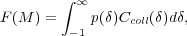 |
(14) |
where p()
d is the PDF of
m(x),
which is given by Equation 2 for the
Gaussian initial density field, and Ccoll is the
probability that any given point x with local overdensity
m(x)
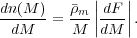
will actually collapse. The mass function can then be derived
as a fraction of the total volume collapsing into halos of mass
(M, M + dM), i.e., dF /
dM, divided by the comoving volume within the initial density
field occupied by each such halo, i.e.,
M /
:
 |
(15) |
In their pioneering model,
Press
& Schechter (1974)
have adopted the ansäz motivated by the spherical collapse model (see
Section 3.1) that any point in space with
m(x)
D+0(z)
c will
collapse into a halo of mass
M by redshift
z: i.e.,
Ccoll() =
 ( -
c), where
is the Heaviside
step function. Note that
m(x)
used above is not the actual initial
overdensity, but the initial overdensity evolved to z = 0 with the
linear growth rate. One can easily check that for a Gaussian initial
density field this assumption gives F(M) = 1/2
erfc[c /
(21/2
(M, z))] =
F().
This line of arguments and assumptions thus leads to an important
conclusion that the abundance of halos of mass M at redshift
z is a universal function of only their peak height
(M, z)
c /
(M, z).
In particular, the fraction of mass in halos per logarithmic interval of
mass in such a model is:
( -
c), where
is the Heaviside
step function. Note that
m(x)
used above is not the actual initial
overdensity, but the initial overdensity evolved to z = 0 with the
linear growth rate. One can easily check that for a Gaussian initial
density field this assumption gives F(M) = 1/2
erfc[c /
(21/2
(M, z))] =
F().
This line of arguments and assumptions thus leads to an important
conclusion that the abundance of halos of mass M at redshift
z is a universal function of only their peak height
(M, z)
c /
(M, z).
In particular, the fraction of mass in halos per logarithmic interval of
mass in such a model is:
 |
(16) |
Clearly, the shape
 ()
in such models is set by the
assumptions of the collapse model. Numerical studies based on
cosmological simulations have eventually revealed that the shape
PS() predicted by the
Press
& Schechter (1974)
model deviates by
()
in such models is set by the
assumptions of the collapse model. Numerical studies based on
cosmological simulations have eventually revealed that the shape
PS() predicted by the
Press
& Schechter (1974)
model deviates by
 50% from the
actual shape measured in cosmological simulations (e.g.,
Klypin et
al. 1995,
Gross et
al. 1998,
Tormen 1998,
Lee &
Shandarin 1999,
Sheth &
Tormen 1999,
Jenkins et
al. 2001).
50% from the
actual shape measured in cosmological simulations (e.g.,
Klypin et
al. 1995,
Gross et
al. 1998,
Tormen 1998,
Lee &
Shandarin 1999,
Sheth &
Tormen 1999,
Jenkins et
al. 2001).
A number of modifications to the original ansäz have been proposed,
which result in
() that more accurately describes
simulation
results. Such modifications are based on the collapse conditions that
take into account asphericity of the peaks in the initial density field
(Monaco 1995,
Audit,
Teyssier & Alimi 1997,
Lee &
Shandarin 1998,
Sheth &
Tormen 2002,
Desjacques
2008)
and stochasticity due to the dependence of the collapse condition on
peak properties other than or
shape (e.g.,
Desjacques
2008,
Maggiore
& Riotto 2010,
de Simone,
Maggiore & Riotto 2011,
Ma et al. 2011,
Corasaniti & Achitouv 2011).
The more sophisticated excursion set models match the simulations more
closely, albeit at the expense of more assumptions and
parameters. There may be also inherent limitations in the accuracy of
such models given that they rely on the strong assumption that one can
parameterize all the factors influencing collapse of any given point
in the initial overdensity field in a relatively compact form. In the
face of complications to a simple picture of peak collapse, as discussed
in Section 3.3, one can indeed expect that the
excursion set ansäze are limited in how accurately they can
ultimately describe the halo mass function.
3.7.2. Calibrations of halo mass function in cosmological simulations
An alternative route to derive predictions for halo abundance
accurately is to calibrate it using large cosmological simulations of
structure formation. Simulations have generally confirmed the
remarkable fact that the abundance of halos can be parameterized via
a universal function of peak height
(Sheth &
Tormen 1999,
Jenkins et
al. 2001,
Evrard et
al. 2002,
White (2002),
Warren et
al. 2006,
Reed et
al. 2007,
Lukic et
al. 2007,
Tinker et
al. 2008,
Crocce et
al. 2010,
Courtin et
al. 2011,
Bhattacharya et al. 2011).
Note that in many studies the linear overdensity for collapse is assumed
to be constant across redshifts
and cosmologies and the mass function is therefore quantified as a
function of -1
- the quantity proportional to
. However, as pointed out by
Courtin et
al. (2011)
it is necessary to include the redshift and cosmology dependence of
c(z)
for an accurate description of the mass function across
cosmologies. Even though
c varies only
by ~ 1-2%, it enters into halo abundance via an exponent and such
small variations can result in variations in the mass function of several
per cent or more.
The main efforts with simulations have thus been aimed at improving
the accuracy of the
() functional form, assessing
systematic uncertainties related to the mass definition, and
quantifying deviations from the universality of
() for
different redshifts and cosmologies. The mass function, and
especially its exponential tail, is sensitive to the specifics of
halo mass definition, a point emphasized strongly in a number of
studies
(Jenkins et
al. 2001,
White 2002,
Tinker et
al. 2008,
Cohn &
White 2008,
Klypin,
Trujillo-Gomez & Primack 2011).
Thus, in precision cosmological analyses using an observed cluster
abundance, care must be taken to ensure that the cluster mass definition
matches that used in the calibration of the halo mass function.
Predictions for the halo abundance as a function of the SO mass for a
variety of overdensities used to define the SO boundaries, accurate to
better than 5-10%
over the redshift interval z = [0,2], were presented by
Tinker et
al. (2008).
In Figure 7 we compare the form of the function
() calibrated through
simulations by different researchers and compared to
() predicted
by the Press-Schechter model, and to the calibration of the functional
form based on the ellipsoidal collapse ansäz by
Sheth, Mo
& Tormen (2001).
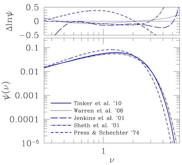 |
Figure 7. The function
|
These calibrations of the mass function through N-body simulations provide the basis for the use of galaxy clusters as tools to constrain cosmological models through the growth rate of perturbations (see the recent reviews by Allen, Evrard & Mantz 2011 and Weinberg et al. 2012). As we discuss in Section 5 below, similar calibrations can be extended to models with non-Gaussian initial density field and models of modified gravity.
Future cluster surveys promise to provide tight constraints on cosmological parameters, thanks to the large statistics of clusters with accurately inferred masses. The potential of such surveys clearly requires a precise calibration of the mass function, which currently represents a challenge. Deviations from universality at the level of up to ~ 10% have been reported (Reed et al. 2007, Lukic et al. 2007, Tinker et al. 2008, Cohn & White 2008, Crocce et al. 2010, Courtin et al. 2011). In principle, a precise calibration of the mass function is a challenging but tractable technical problem, as long as it only requires a large suite of dissipationless simulations for a given set of cosmological parameters, and an optimal interpolation procedure (e.g., Lawrence et al. 2010).
A more serious challenge is the modelling of uncertain effects of baryon physics: baryon collapse, dissipation, and dynamical evolution, as well as feedback effects related to energy release by the SNe and AGN, may lead to subtle redistribution of mass in halos. Such redistribution can affect halo mass and thereby halo mass function at the level of a few per cent (Rudd, Zentner & Kravtsov 2008, Stanek, Rudd & Evrard 2009, Cui et al. 2011, although the exact magnitude of the effect is not yet certain due to uncertainties in our understanding of the physics of galaxy formation in general, and the process of condensation and dynamical evolution in clusters in particular.
Galaxy clusters are clustered much more strongly than galaxies
themselves. It is this strong clustering discovered in the early 1980s
(Klypin
& Kopylov 1983,
Bahcall
& Soneira 1983)
that led to the development of the concept of bias in the context of
Gaussian initial density perturbation field
(Kaiser 1984).
Linear bias of halos is the coefficient between the overdensity of halos
within a given sufficiently large region and the overdensity of matter
in that region:
h =
b, with b
defined as
the bias parameter. For the Gaussian perturbation fields, local linear
bias is independent of scale
(Scherrer
& Weinberg (1998)),
such that the large-scale power spectrum and correlation function on
large scales can be expressed in terms of the corresponding quantities
for the underlying matter distribution as
Phh(k)
= b2 Pmm(k) and
 hh(r) = b2
mm(r), respectively. As we discuss in
Section 5, this
is not true for non-Gaussian initial perturbation fields
(Dalal et
al. 2008)
or for models with scale-dependent linear growth rate
(Parfrey,
Hui & Sheth 2011),
in which cases the linear bias is generally scale-dependent.
hh(r) = b2
mm(r), respectively. As we discuss in
Section 5, this
is not true for non-Gaussian initial perturbation fields
(Dalal et
al. 2008)
or for models with scale-dependent linear growth rate
(Parfrey,
Hui & Sheth 2011),
in which cases the linear bias is generally scale-dependent.
In the context of the hierarchical structure formation, halo bias is
closely related to the overall abundance of halos discussed above, as
illustrated by the "peak-background split" framework
(Kaiser 1984,
Cole &
Kaiser 1989,
Mo & White
1996,
Sheth &
Tormen 1999),
in which the linear halo bias is obtained by considering a Lagrangian
patch of volume V0, mass
M0, and overdensity
0 at some early
redshift z0. The bias is calculated by requiring that
the abundance
of collapsed density peaks within such a patch is described by the same
function (p)
as the mean abundance of halos in the Universe, but with peak height
p appropriately
rescaled with respect to
the overdensity of the patch and relative to the rms fluctuations on
the scale of the patch. Thus, the functional form of the bias
dependence on halo mass, bh(M), depends on the
functional form of
the mass function explicitly in this framework. Simulations show that
the peak-background split model provides a fairly accurate (to ~
20%) prediction for the linear halo bias
(Tinker et
al. 2010).
Another line of argument illustrating the close connection between the
halo abundance and bias is the fact that if one assumes that all of the
mass is in the collapsed halos, as is done for example in the halo
models
(Cooray
& Sheth 2002),
the requirement that matter in the
Universe is not biased against itself implies that
b()
g()
dln = 1 (e.g.,
Seljak 2000),
where g()
|
dln /
dlnM|-1
() (see eq.16). This integral
constraint requires that the form of the bias function
b() is changed whenever
() changes.
Incidentally, the close connection between
b() and
() implies that if
() is a universal function, then
the bias b() should be
a universal function as well.
The function b()
recently calibrated for the SO-defined halos
of different overdensities using a suite of large
cosmological simulations with accuracy
5% and satisfying
the integral constraint
(Tinker et
al. 2010)
is shown in Figure 8 for halos defined using an
overdensity
of = 200 with
respect to the mean. This calibration of the bias is
compared to the corresponding prediction of the
Press
& Schechter (1974)
and the
Sheth, Mo
& Tormen (2001)
ansäze. The figure shows that
b() is a rather weak
function of at
< 1, but steepens
substantially for rare peaks of
> 1. It also shows that
the rarest clusters ( ~ 5)
in the
Universe can have the amplitude of the correlation function or power
spectrum that is two orders of magnitude larger than the clustering
amplitude of the galaxy-sized halos
(
1).
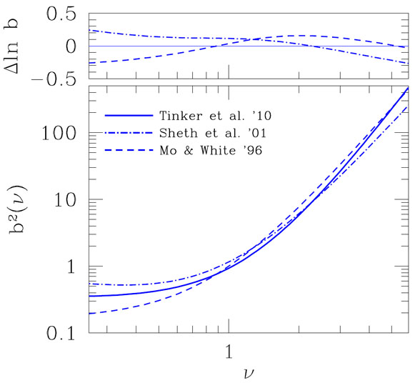 |
Figure 8. The square of the bias,
b2( |
3.9. Self-similar evolution of galaxy clusters
In the previous sections we have considered processes that govern the collapse of matter during cluster formation, the transition to equilibrium and the equilibrium structure of matter distribution in collapsed halos. In the following sections, we consider baryonic processes that shape the observable properties of clusters, such as their X-ray luminosity or the temperature of the ICM. However, before we delve into the complexities of such physical processes, it is instructive to introduce the simplest models based on assumptions of self-similarity, in which the number of control parameters is minimal. We discuss the assumptions and predictions of the self-similar model in some detail because parametric scalings that it predicts are in wide use to interpret results from both cosmological simulations of cluster formation and observations.
3.9.1. Self-similar model: assumptions and basic expectations
The self-similar model developed by
Kaiser (1986)
makes three key assumptions. The first assumption is that clusters form via
gravitational collapse from peaks in the initial density field in
an Einstein-de-Sitter Universe,
m = 1.
Gravitational collapse in such a
Universe is scale-free, or self-similar. The second assumption
is that the amplitude of density fluctuations is a power-law function of
their size,
(k)
k3+n. This means that initial
perturbations also do not have a preferred scale (i.e., they are
scale-free or self-similar). The third assumption is that the physical
processes that shape the properties of forming clusters do not introduce
new scales in the problem. With these assumptions the problem has only
two control parameters: the normalization of the power spectrum of the
initial density perturbations at an initial time, ti,
and its
slope, n. Properties of the density field and halo population at
t > ti (or corresponding redshift
z < zi), such as typical halo masses that
collapse or halo abundance as a function of mass, depend only on these
two parameters. One can choose any suitable variable that depends on
these two parameters as a characteristic variable for a given
problem. For evolution of halos and their abundance, the commonly used
choice is to define the characteristic nonlinear mass,
MNL
(see Section 3.1), which encapsulates such
dependence. The halo properties and halo abundance then become universal
functions of µ
M /
MNL in such model. Thus, for example, clusters with masses
M1(z1) and
M2(z2) that
correspond to the same ratio M1(z1)
/ MNL(z1) =
M2(z2) /
MNL(z2)
have the same dimensionless properties, such as gas fraction or
concentration of their mass distribution.
As we have discussed above, in more general cosmologies the halo
properties and mass function should be universal functions of the peak
height , which encapsulates
the dependence on the shape and normalization of the power spectra for
general, non power-law shapes of the fluctuation spectrum.
3.9.2. The Kaiser model for cluster scaling relations
In this Section, we define cluster mass to be the mass within the sphere
of radius R, encompassing characteristic density contrast,
, with respect to
some reference density
r
(usually either
cr or
m):
M =
(4 / 3)
r
R3. In this definition,
radius and mass are directly related and interchangeable. The model
assumes spherical symmetry and that the ICM is in equilibrium within the
cluster gravitational potential, so that the HE equation (eq. 9)
holds. The mass M(< R) derived from the HE equation is
proportional to T(R)R and the sum of the
logarithmic slopes of the gas density and temperature profiles at
R. In addition to the assumptions about self-similarity
discussed above, a key assumption made in the model by
Kaiser (1986)
is that these slopes are independent of M, so that
 |
(17) |
Note that formally the quantity T appearing in the above
equation is the temperature measured at R, whereas some average
temperature at smaller radii is usually measured in
observations. However, if we parameterize the temperature profile as
T(r) = T∗
T(x), where T∗ is the
characteristic temperature and
T is the dimensionless profile as a function of dimensionless radius
x r /
R, and we assume that
T(x) is independent of M, any
temperature averaged over the same fraction of radial range
[x1, x2] will scale as
T∗
T(R).
The latter is not strictly true for the "spectroscopic" temperature,
TX, derived by fitting an observed X-ray spectrum to a
single-temperature bremsstrahlung model
(Mazzotta
et al. 2004,
Vikhlinin
2006),
although in practice deviations
of TX from the expected behavior for
T∗ are small.
The gas mass within R can be computed by integrating over the gas
density profile, which, by analogy with temperature, we parameterize as
g(r) =
g∗
g(x), where
g∗ is the characteristic density and
g
is the dimensionless profile. The gas mass
within R can then be expressed as
 |
(18) |
The latter proportionality is assumed in the
Kaiser (1986)
model, which means that g∗ and
Ig are assumed to be independent of
M. Note that g∗
r, so
r does
not enter the Mg - M relation.
Using the scalings of Mg and T with mass, we can construct other cluster properties of interest, such as the luminosity of ICM emitted due to its radiative cooling. Assuming that the ICM emission is due to the free-free radiation and neglecting the weak logarithmic dependence of the Gaunt factor on temperature, the bolometric luminosity can be written as (e.g., Sarazin 1986):
 |
(19) |
We omit
r
in these equations for clarity; it suffices to remember that
r
enters into the scaling relations exactly as
. Note that the
bolometric luminosity of a cluster is not
observable directly, and the X-ray luminosity in soft band (e.g.,
0.5-2 keV), LXs, is frequently used. Such soft band X-ray
luminosity is almost insensitive to temperature at T > 2 keV
(Fabricant & Gorenstein 1983),
as can be easily verified with a plasma emission code), so that its
temperature dependence can be neglected. LXs then
scales as:
 |
(20) |
At temperatures T < 2 keV temperature dependence is more complicated both for the bolometric and soft X-ray emissivity due to significant flux in emission lines. Therefore, strictly speaking, for lower mass systems the above L - M scaling relations are not applicable, and scaling of the emissivity with temperature needs to be calibrated separately taking also into account the ICM metallicity. The same is true for luminosity defined in some other energy band or for the bolometric luminosity.
Another quantity of interest is the ICM "entropy" defined in X-ray analyses as
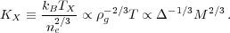 |
(21) |
where ne is the electron number density.
Finally, the quantity, Y = MgT where gas
mass and temperature
are measured within a certain range of radii scaled to
R,
is used to characterize the ICM in the analyses of
SZ and X-ray observations. This
quantity is expected to be a particularly robust proxy of the cluster
mass (e.g.,
da Silva et
al. 2004,
Motl et
al. 2005,
Nagai 2006,
Kravtsov,
Vikhlinin & Nagai 2006,
Fabjan et
al. 2011,
see also discussion in Section 4)
because it is proportional to the global thermal energy of ICM. Using
Equations 18 and 17 the scaling of Y with mass
in the self-similar model is
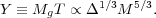 |
(22) |
Note that the redshift dependence in the normalization of the scaling
relations introduced above is due solely to the particular SO
definition of mass and associated redshift dependence of
r. In
m
1
cosmologies, there is a choice of
either defining the mass relative to the mean matter density or
critical density (Section 3.6.2). This specific,
arbitrary choice determines the specific redshift dependence of
the observable-mass relations. It is clear that this evolution due to
(z) factors
has no deep physical meaning. However,
the absence of any additional redshift dependence in the
normalization of the scaling relations is just the consequence of the
assumptions of the
Kaiser (1986)
model and is a physical reflection of these assumptions.
Extra evolution can, therefore, be expected if one or more of the assumptions of the self-similar model is violated. This can be due to either actual physical processes that break self-similarity or the fact that some of the model assumptions are not accurate. We discuss physical processes that lead to the breaking of self-similarity in subsequent sections. Here below we first consider possible deviations that may arise because assumptions of the Kaiser model do not hold exactly, i.e. deviations not ascribed to physical processes that explicitly violate self-similarity.
3.9.3. Extensions of the Kaiser model
Going back to equations 17 and 18, we note that
the specific scaling of T
M2/3 and Mg
M will only
hold, if the assumption that the dimensionless temperature and gas
density profiles, T(x) and
g(x), are independent of M
holds. In practice, however, some mass dependence of these profiles is
expected. For example, if the concentration of the gas distribution
depends on mass similarly to the concentration of the DM profile
(Ascasibar
et al. 2006),
the weak mass dependence of DM concentration implies weak mass
dependence of g(x)
and T(x). Indeed, concentration depends on mass even in
purely self-similar models
(Cole &
Lacey 1996,
Navarro,
Frenk & White 1997).
These dependencies imply that predictions of the Kaiser model may not
describe accurately even the purely self-similar evolution. This is
evidenced by deviations of scaling relation evolution from these
predictions in hydrodynamical simulations of cluster formation even in
the absence of any physical processes that can break self-similarity
(e.g.,
Nagai 2006,
Stanek et
al. 2010).
In addition, the characteristic gas density,
g∗, may be mildly
modified by a mass-dependent, non self-similar process during some
early stage of evolution. If such a process does not introduce a
pronounced mass scale and is confined to some early epochs (e.g., owing
to shutting off of star formation in cluster galaxies due to AGN
feedback and gas accretion suppression), then subsequent evolution may
still be described well by the self-similar model. The Kaiser model is
just the simplest specific example of a more general class of
self-similar models, and can therefore be extended to take into
account deviations described above.
For simplicity, let us assume that the scalings of gas mass and gas mass fraction against total mass can be expressed as a power law of mass:
 |
(23) |
This does not violate the self-similarity of the problem per se, as long
as dimensionless properties of an object,
such as fg, remain a function of only the
dimensionless mass µ(z)
M /
MNL(z). This means that the normalization of the
Mg-M relation must scale as Cg
MNL-g during the
self-similar stages of evolution, such that
 |
(24) |
Note that self-similarity requires that the slope
g does not
evolve with redshift.
By analogy with the Mg-M relation, we can assume that the T-M relation can be well described by a power law of the form
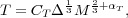 |
(25) |
where t
describes mild deviation from the scaling due, e.g., to mild dependence
of gas and temperature profile slopes in the HE equation. The
dimensionless quantities involving temperature T can be
constructed using ratios of T with TNL =
(µ mp /
kB)G MNL /
RNL
1/3
MNL2/3. As before for
the gas fraction, requirement that such dimensionless ratio depends only
on µ requires Ct
MNL-t so that
 |
(26) |
Other observable-mass scaling relations can be constructed in the
manner similar to the derivation of the original relations
above. These are summarized below for the specific choice of
r
c
cr(z)
h2E2(z):
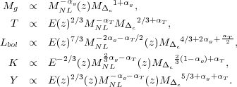 |
(27) (28) (29) (30) (31) |
In all of the relations one can, of course, recover the original
relations by setting
g
= t = 0.
The observable-mass relations can be used to predict
observable-observable relations by eliminating mass from the
corresponding relations above.
Note that the evolution of scaling relations in this extended model
arises both from the redshift dependence of
(z)
r(z) and
from the extra redshift dependence due to factors involving
MNL.
The practical implication is that if measurements show that
g
0
and/or t
0 at some redshift, the
original Kaiser scaling
relations are not expected to describe the evolution, even if the
evolution is self-similar. Instead, relations given by
Equations 27-31 should be used. Note that at
z 0,
observations indicate that within the radius
r500 enclosing overdensity
c = 500,
g
0.1-0.2, while
t
0.-0.1. Therefore,
the extra evolution compared to the
Kaiser model predictions due to factors involving
g and, to a
lesser degree, factors involving
t is
expected. Such evolution, consistent with predictions of the above
equations, is indeed observed both in simulations (see, e.g., Fig. 10 in
Vikhlinin
et al. 2009b)
and in observations
(Lin et
al. 2012, although see
Böhringer, Dolag & Chon 2012).
In practice, evolution of the scaling relations can be quite a bit more
complicated than the evolution predicted by the above equations. The
complication is not due to any deviation from self-similarity but rather
due to specific mass definition and the fact that cluster formation is
an extended process that is not characterized by a single collapse
epoch. Some clusters evolve only mildly after their last major
merger. However, the mass of such clusters will change with z
even if their potential does not change, simply because mass definition
is tied to a reference density that changes with expansion of the
Universe and because density profiles of clusters extends smoothly well
beyond the virial radius. Any observable property of clusters that has
radial profile differing from the mass profile, but which is measured
within the same
R,
will change differently than
mass with redshift. As a simplistic toy model, consider a population of
clusters that does not evolve from z = 1 to z = 0. Their
X-ray luminosity is mostly due to the ICM in the central regions of
clusters and it is not sensitive to the outer boundary of integration as
long as it is sufficiently large. Thus, X-ray luminosity of such a
non-evolving population will not change with z, but masses
M
of clusters will increase with decreasing
z as the reference density used to define the cluster boundary
decreases. Normalization of the LX -
M
relation will thus
decrease with decreasing redshift simply due to the definition of
mass. The strength of the evolution will be determined by the slope of
the mass profile around
R,
which is weakly
dependent on mass. Such an effect may, thus, result in the evolution of
both the slope and normalization of the relation. In this respect,
quantities that have radial profiles most similar to the total mass
profile (e.g., Mg, Y) will suffer the least
from such spurious evolution.
Finally, we note again that in principle for general non power-law
initial perturbation spectra of the CDM models the scaling with M
/ MNL needs to be replaced with scaling with the peak
height . For clusters within a
limited mass range, however, the
power spectrum can be approximated by a power law and thus a
characteristic mass similar to MNL can be constructed,
although such mass should be within the typical mass range of the
clusters. The latter is not true for MNL, which is
considerably smaller than typical cluster mass at all z.
3.9.4. Practical implications for observational calibrations of scaling relations
In observational calibrations of the cluster scaling relations, it is
often necessary to rescale between different redshifts either to bring
results from the different z to a common redshift, or because the
scaling relation is evaluated using clusters from a wide range of
redshifts due to small sample size. It is customary to use predictions
of the Kaiser model to carry out such rescaling to take into account the
redshift dependence of
(z). In this
context, one should
keep in mind that these predictions are approximate due to the
approximate nature of some of the assumptions of the model, as discussed
above. Inaccuracies introduced by such scalings may, for example, then
be incorrectly interpreted as intrinsic scatter about the scaling
relation.
In addition, because the
(z) factors
are a result of an arbitrary mass definition, they should not be
interpreted as physically meaningful factors describing evolution of
mass. For example, in the T-M relation, the
1/3 factor in
Equation 17 arises due to the dimensional M/R factor
of the HE equation. As such, this factor does not change even if the
power-law index of the T-M relation deviates from 2/3, in
which case the relation has the form T
1/3
M2/3+t. In other words, if one fits for the
parameters of this relation, such as normalization A and slope
B, using measurements of temperatures and masses for a sample of
clusters spanning a range of redshifts, the proper parameterization of
the fit should be
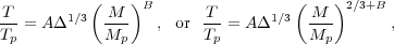 |
(32) |
where Tp and Mp are appropriately
chosen pivots. The parameterization T / Tp =
A(1/3 M /
Mp)B that is sometimes adopted in
observational analyses is not correct in the context of the
self-similar model. In other words, only the observable quantities
should be rescaled by the
r
factors, and not the mass. Likewise, only the
r
factors actually predicted by the Kaiser model
should be present in the scalings. For example, no such factor is
predicted for the Mg-M relation and therefore
the gas and total masses of clusters at different redshifts should not
be scaled by r
factors in the fits of this relation.
Finally, we note that observational calibrations of the
observable-mass scaling relations generally depend on the distances to
clusters and are therefore cosmology dependent. Such dependence arises
because distances are used to convert observed angular scale to physical
scale within which an "observable" is defined,
R =  dA(z)
h-1,
or to convert observed flux f to
luminosity, L = 4
fdL(z),
where dA(z) and dL(z)
= dA(z)(1 + z)2 are the
angular diameter distance and luminosity distance, respectively.
Thus, if the total mass M of a cluster is measured using the HSE
equation, we have MHE
TR
dA
h-1. The same scaling is expected for the mass derived
from the weak lensing shear profile measurements.
dA(z)
h-1,
or to convert observed flux f to
luminosity, L = 4
fdL(z),
where dA(z) and dL(z)
= dA(z)(1 + z)2 are the
angular diameter distance and luminosity distance, respectively.
Thus, if the total mass M of a cluster is measured using the HSE
equation, we have MHE
TR
dA
h-1. The same scaling is expected for the mass derived
from the weak lensing shear profile measurements.
If the gas mass is measured from the X-ray flux from a volume
V
R3
3
dA3, which scales as
f = LX /
(4
dL2)
g2 V /
dL2
Mg2 /
(VdL2)
Mg2 /
(
dL2
dA3) and where f and
are
observables, gas mass then scales with distance as
Mg
dL
dA3/2
h5/2. This dependence can be exploited to
constrain cosmological parameters, as in the case of X-ray
measurements of gas fractions in clusters
(Ettori,
Tozzi & Rosati 2003,
Allen et
al. 2004,
LaRoque et
al. 2006,
Allen et
al. 2008,
Ettori et
al. 2009)
or abundance evolution of clusters as a function of their observable
(e.g.,
Vikhlinin
et al. 2009c).
In this respect, the Mg-M
relation has the strongest scaling with distance and cosmology, whereas
the scaling of the T-M relation is the weakest (e.g., see
discussion by
Vikhlinin
et al. 2009b).
3.10. Cluster formation and Thermodynamics of the Intra-cluster gas
Gravity that drives the collapse of the initial large-scale density peaks affects not only the properties of the cluster DM halos, but also the thermodynamic properties of the intra-cluster plasma. The latter are also affected by processes related to galaxy formation, such as cooling and feedback. Below, we discuss the thermodynamic properties of the ICM resulting from gravitational heating, radiative cooling, and stellar and AGN feedback during cluster formation.
3.10.1. Gravitational collapse of the intra-cluster gas
The diffuse gas infalling onto the DM-dominated potential wells of clusters converts the kinetic energy acquired during the collapse into thermal energy via adiabatic compression and shocks. As gas settles into HE, its temperature approaches values close to the virial temperature corresponding to the cluster mass. In the spherically symmetric collapse model of Bertschinger (1985), supersonic accretion gives rise to the expanding shock at the interface of the inner hydrostatic gas with a cooler, adiabatically compressed, external medium. Real three-dimensional collapse of clusters is more complicated and exhibits large deviations from spherical symmetry, as accretion proceeds both in a quasi-spherical fashion from low-density regions and along relatively narrow filaments. The gas accreting along the latter penetrates much deeper into the cluster virial region and does not undergo a shock at the virial radius (see Fig. 9). The strong shocks are driven not just by the accretion of gas from the outside but also "inside-out" during major mergers (e.g., Poole et al. 2007).
 |
Figure 9. Left panel: map of the shocked
cells identified by the
divergence of velocity colored by the local shock Mach number and
turbulent gas velocity field (streamlines) in a slice of the
simulation box 7.5 Mpc on a
side and depth of 18 kpc at z = 0.6, for a simulated cluster that
reaches a mass of ~ 2 × 10¹⁴
M |
The shocks arising during cluster formation can be classified into two
broad categories: strong external shocks surrounding filaments and the
virialized regions of DM halos and weaker internal shocks, located
within the cluster virial radius (e.g.,
Pfrommer et
al. 2006,
Skillman et
al. 2008,
Vazza et
al. 2009).
The strong shocks arise in the high-Mach number flows of the intergalactic
gas, whereas weak shocks arise in the relatively low-Mach number flows
of gas in filaments and accreting groups, which was pre-heated at
earlier epochs by the strong shocks surrounding filaments or external
groups. The left panel of Figure 9 shows these two
types of shocks in a map of the shocked cells identified in a
cosmological adaptive mesh refinement simulation of a region
surrounding a galaxy cluster (from
Vazza et
al. 2009),
along with the gas velocity field. This map highlights the strong external
shocks, characterized by high Mach numbers
 > 30, surrounding
the cluster at several virial radii from the cluster center, and
weaker internal shocks, with
2-3. The cluster is
shown at the epoch immediately following a major merger, which
generated substantial velocities of gas within virial radius. As we
discuss in Section 4 below, incomplete
thermalization of these gas motions is one of the main sources of
non-thermal pressure support in the ICM.
> 30, surrounding
the cluster at several virial radii from the cluster center, and
weaker internal shocks, with
2-3. The cluster is
shown at the epoch immediately following a major merger, which
generated substantial velocities of gas within virial radius. As we
discuss in Section 4 below, incomplete
thermalization of these gas motions is one of the main sources of
non-thermal pressure support in the ICM.
The right panel of Figure 9 shows the
distribution of the kinetic energy processed by shocks, as a function of
the local shock Mach number, for different redshifts
(Skillman
et al. 2008).
The figure shows that a large fraction of the
kinetic energy is processed by weak internal shocks and this fraction
increases with decreasing redshift as more and more of the accreting
gas is pre-heated in filaments. Yet, the left panel of
Fig. 9 highlights that
large- shocks
surround virialized halos in such a way that most gas particles
accreted in a galaxy cluster must have experienced at least one strong
shock in their past.
Becasuse gravity does not have a characteristic length scale, we expect the predictions of the self-similar model, presented in Section 3.9, to apply when gravitational gas accretion determines the thermal properties of the ICM. The scaling relations and their evolution predicted by the self-similar model are indeed broadly confirmed by the non-radiative hydrodynamical simulations that include only gravitational heating (e.g., Navarro, Frenk & White 1995, Eke, Navarro & Frenk 1998, Nagai, Kravtsov & Vikhlinin 2007), although some small deviations arising due to small differences in the dynamics of baryons and DM were also found (Ascasibar et al. 2006, Nagai 2006, Stanek et al. 2010).
As discussed in Section 2, observations
carried out with the Chandra and
XMM-Newton telescopes during the
past decade showed that the outer regions of clusters (r
r2500) exhibit self-similar scaling, whereas the core
regions exhibit strong deviations from self-similarity. In particular, gas
density in the core regions of small-mass clusters is lower than
expected from self-similar scaling of large-mass systems. These
results indicate that some additional non-gravitational processes are
shaping properties of the ICM. We review some of these processes
studied in cluster formation models below.
3.10.2. Phenomenological pre-heating models
The first proposed mechanism to break self-similarity was
high-redshift (zh
3) pre-heating by
non-gravitational sources of energy, presumably by a combined action of
the AGN and stellar feedback
(Kaiser 1991,
Evrard &
Henry 1991).
The specific extra heating energy per unit mass, Eh,
defines the temperature scale T*
Eh / kB, such that clusters with
virial temperature Tvir >
T* should be left almost unaffected by the extra
heating, whereas in smaller clusters with Tvir <
T* gas accretion is suppressed. As a result,
gas density is relatively lower in lower massive systems, especially at
smaller radii, while their entropy will be higher.
Both analytical models (e.g. Tozzi & Norman 2001, Babul et al. 2002, Voit et al. 2003) and hydrodynamical simulations (e.g. Bialek, Evrard & Mohr 2001, Borgani et al. 2002, Muanwong et al. 2002) have demonstrated that with a suitable pre-heating prescription and typical heating injection of Eh ~ 0.5-1 keV per gas particle self-similarity can be broken to the degree required to reproduce observed scaling relations. Studies of the possible feedback mechanisms show that such amounts of energy cannot be provided by SNe (e.g., Kravtsov & Yepes 2000, Renzini 2000, Borgani et al. 2004, Kay et al. 2007, Henning et al. 2009), and must be injected by the AGN population (e.g., Wu, Fabian & Nulsen 2000, Lapi, Cavaliere & Menci 2005, Bower, McCarthy & Benson 2008) or by some other unknown source.
However, regardless of the actual sources of heating, strong
widespread heating at high redshifts would conflict with the observed
statistical properties of the
Lyman- forest
(Shang, Crotts
& Haiman 2007,
Borgani
& Viel 2009).
Moreover, hydrodynamical simulations have demonstrated that simple
pre-heating models predict large isentropic cores (e.g.,
Borgani et
al. 2005,
Younger
& Bryan 2007)
and shallow pressure profiles
(Kay et
al. 2012).
This is at odds with the entropy and pressure profiles of real clusters
which exhibit smoothly declining entropy down to r ~ 10-20 kpc
(e.g.,
Cavagnolo
et al. 2009,
Arnaud et
al. 2010).
3.10.3. The role of radiative cooling
The presence of galaxies in clusters and low levels of the ICM entropy in cluster cores are a testament that radiative cooling has operated during cluster formation in the past and is an important process shaping thermodynamics of the core gas at present. Therefore, in general radiative cooling cannot be neglected in realistic models of cluster formation. Given that cooling generally introduces new scales, it can break self-similarity of the ICM even in the absence of heating (Voit & Bryan 2001). In particular, cooling removes low-entropy gas from the hot ICM phase in the cluster cores, which is replaced by higher entropy gas from larger radii. Somewhat paradoxically, the cooling thus leads to an entropy increase of the hot, X-ray emitting ICM phase. This effect is illustrated in Figure 10, which shows the entropy maps in the simulations of the same cluster with and without cooling. In the absence of cooling (left panel), the innermost region of the cluster is filled by low-entropy gas. Merging substructures also carry low-entropy gas, which generates comet-like features by ram-pressure stripping, and is hardly mixed in the hotter ambient of the main halo. In the simulation with radiative cooling (right panel), most of the low-entropy gas associated with substructures and the central cluster region is absent, and most of the ICM has a relatively high entropy.
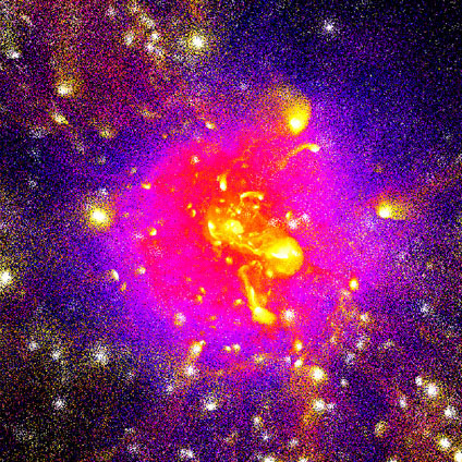 |
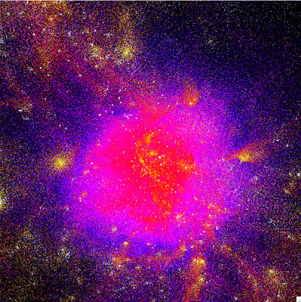 |
Figure 10. Maps of entropy in
cosmological hydrodynamical simulations of a galaxy cluster of mass
M500
|
|
A more quantitative analysis of the entropy distribution for these
simulated clusters is shown in Figure 11, in which
the entropy profiles of clusters simulated with inclusion of different
physical processes are compared with the baseline analytic spherical
accretion model; this model predicts the power-law entropy profile
K(r)
r1.1 (e.g.
Tozzi &
Norman 2001,
Voit 2005).
The figure shows that the entropy profile in the simulation with radiative
cooling is significantly higher than that of the non-radiative
simulation. The difference in entropy is as large as an order of
magnitude in the inner regions of the cluster and is greater by a
factor of two even at r500.
Interestingly, the predicted level of entropy at r ~
r2500 - r500 in the simulations with
cooling (but no significant heating) is consistent with the ICM entropy
inferred from X-ray observations. However, this agreement is likely to
be spurious because it is achieved with the amount of cooling that
results in conversion of
40% of
the baryon mass in clusters into stars and cold gas, which is
inconsistent with observational measurements of cold fraction varying from
 20-30% for small-mass,
X-ray-emitting clusters to
10% for massive
clusters (see Section 2).
20-30% for small-mass,
X-ray-emitting clusters to
10% for massive
clusters (see Section 2).
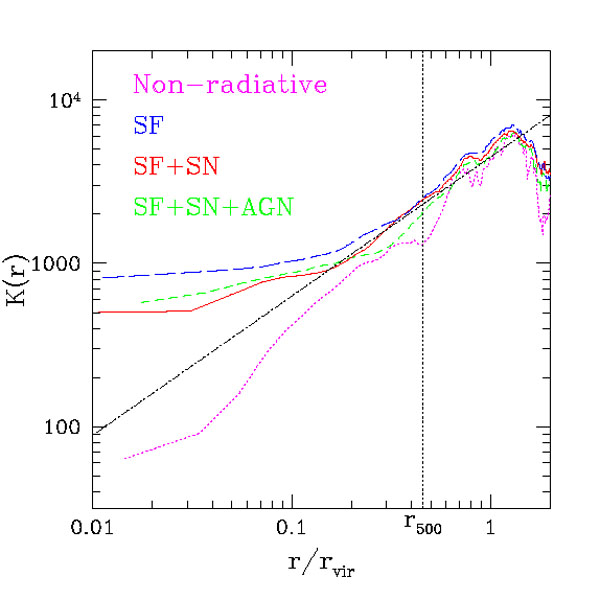 |
Figure 11. Radial profiles of entropy (in
units of kiloelectronvolt-centimeters squared) for the same simulations
whose entropy maps are shown in
Figure 10. Magenta dotted, long-dashed blue,
continuous red, and short-dashed green curves refer to the
non-radiative simulation and to the three radiative simulations
including only cooling and star formation, including also the effect
of galactic ejecta from supernova, and including also the effect of
AGN feedback, respectively. The dot-dashed line shows the power-law
entropy profile with slope K(r)
|
Finally, note that inclusion of cooling in simulations with pre-heating discussed above usually results in problematic star-formation histories. In fact, if pre-heating takes place at a sufficiently high redshift, clusters exhibit excessive cooling at lower redshifts, as pre-heated gas collapses and cools at later epochs compared to the simulations without pre-heating (e.g. Tornatore et al. 2003). These results highlight the necessity to treat cooling and heating processes simultaneously using heating prescriptions that can realistically reproduce the heating rate of the ICM gas as a function of cosmic time. We discuss efforts in this direction next.
3.10.4. Thermodynamics of the intracluster medium with stellar and active galactic nuclei feedback
The results discussed above strongly indicate that, in order to reproduce the overall properties of clusters, cooling should be modelled together with a realistic prescription for non-gravitational heating. This is particularly apparent in the cluster cores, where a steady heating is required to offset the ongoing radiative cooling observed in the form of strong X-ray emission (see, e.g., Peterson & Fabian 2006). Studies of the feedback processes in clusters is one of the frontiers in cluster formation modelling. Although we do not yet have a complete picture of the ICM heating, a number of interesting and promising results have been obtained.
In Figure 11, the solid line shows the effect of the SN feedback on the entropy profile. In these simulations, the kinetic feedback of SNe is included in the form of galactic winds carrying the kinetic energy comparable to all of the energy released by Type-II SNe expected to occur according to star formation in the simulation. This energy partially compensates for the radiative losses in the central regions, which leads to a lower level of entropy in the core. However, the core ICM entropy in these simulations is still considerably higher than observed (e.g., Sun et al. 2009). The inefficiency of the SN feedback in offsetting the cooling sufficiently is also evidenced by temperature profiles.
Figure 4 (from
Leccardi
& Molendi 2008)
compares the observed temperature profiles of a sample of local clusters
with results from simulations that include the SN feedback. The figure
shows that simulations reproduce the observed temperature profile at
r
0.2r180. The overall shape of the profile at these large
radii is reproduced by simulations including a wide range of physical
processes, including non-radiative simulations (e.g.,
Loken et
al. 2002,
Borgani et
al. 2004,
Nagai,
Kravtsov & Vikhlinin 2007).
At large radii, however, the observed and predicted profiles do not
match: The profiles in simulated clusters continue to increase to the
smallest resolved radii, whereas the observed profiles reach a maximum
temperature Tmax
2T180 and then decrease with
decreasing radius to temperatures of ~ 0.1-0.3Tmax. The
high temperatures of the central gas reflects its high entropy and is
due to the processes affecting the entropy, as discussed above.
Another indication that the SN feedback alone is insufficient is the
fact that the stellar mass of the BCGs in simulations that include
only the feedback from SNe is a factor of two to three larger than the
observed stellar masses. For example, in the simulated clusters shown
in figure 10, the baryon fraction in stars within
r500 decreases from
40% in simulations
without SN feedback to
30%, which is still a factor of two larger than
observational measurements. The overestimate of the stellar mass is
reflected in the overestimate of the ICM metallicity in cluster cores
(e.g.,
Borgani et
al. 2008
and references therein).
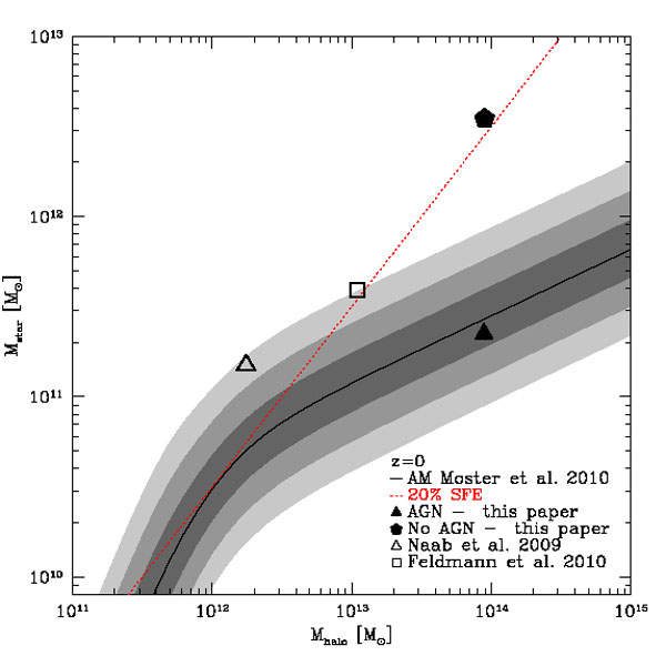 |
Figure 12. Comparison of the relation
between stellar mass and total
halo mass as predicted by cosmological hydrodynamical simulations of
four early-type galaxies (symbols) (from
Martizzi,
Teyssier & Moore 2012).
The open triangle and square refer to the simulations presented by
Naab,
Johansson & Ostriker (2009)
and by
Feldmann et
al. (2010),
both based on the smoothed
particle hydrodynamics codes and not including AGN feedback. The
filled symbols refer to the simulations by
Martizzi,
Teyssier & Moore (2012)
with the brightest cluster galaxies
forming at the center of a relatively poor cluster carried out with
an AMR code, both including (triangle) and excluding (pentagon) AGN
feedback. The red dotted line represents the relation expected for
20% efficiency in the conversion of baryons into stars. The solid
black line is the prediction from
Moster et
al. (2010)
of a model in which dark matter halos are populated with stars in such a
way as to reproduce the observed stellar mass function. The grey shaded
areas represent the 1-, 2- and
3- |
Different lines of evidence indicate that energy input from the AGN in the central cluster galaxies can provide most of the energy required to offset cooling (see McNamara & Nulsen 2007 for a comprehensive review). Because the spatial and temporal scales resolved in cosmological simulations are larger than those relevant for gas accretion and energy input, the AGN energy feedback can only be included via a phenomenological prescription. Such prescriptions generally model the feedback energy input rate by assuming the Bondi gas accretion rate onto the SMBHs, included as the sink particles, and incorporate a number of phenomenological parameters, such as the radiative efficiency and the feedback efficiency, which quantify the fraction of the radiated energy that thermally couples to the surrounding gas (e.g., Springel, Di Matteo & Hernquist 2005). The values of these parameters are adjusted so that simulations reproduce the observed relation between black hole mass and the velocity dispersion of the host stellar bulge (e.g., Marconi & Hunt 2003). An alternative way of implementing the AGN energy injection is the AGN-driven winds, which shock and heat the surrounding gas (e.g., Omma et al. 2004, Dubois et al. 2011, Gaspari et al. 2011).
In general, simulations of galaxy clusters based on different variants of these models have shown that the AGN feedback can reduce star formation in massive cluster galaxies and reduce the hot gas content in the poor clusters and groups, thereby improving agreement with the observed relation between X-ray luminosity and temperature (e.g., Sijacki et al. 2007, Puchwein, Sijacki & Springel 2008). Figure 12 (from Martizzi, Teyssier & Moore 2012) shows that simulations with the AGN feedback results in stellar masses of the BCGs that agree with the masses required to match observed stellar masses of galaxies and masses of their DM halos predicted by the models. The figure also shows that stellar masses are over-predicted in the simulations without the AGN feedback. Incidentally, the large-scale winds at high redshifts and stirring of the ICM in cluster cores by the AGN feedback also help to bring the metallicity profiles into cluster simulations in better agreement with observations (Fabjan et al. 2010, McCarthy et al. 2010).
Although results of simulations with the AGN feedback are promising, simulations so far have not been able to convincingly reproduce the observed thermal structure of cool cores. As an example, Figure 11 shows that the entropy profiles in such simulations still develop large constant entropy core inconsistent with observed profiles. Interestingly, the adaptive mesh refinement simulations with jet-driven AGN feedback by Dubois et al. (2011) reproduce the monotonically decreasing entropy profiles inferred from observations. However, such agreement only exists if radiative cooling does not account for the metallicity of the ICM; in simulations that take into account the metallicity dependence of the cooling rates the entropy profile still develosp a large constant entropy core.
The presence of a population of relativistic particles in AGN-driven
high-entropy bubbles has been suggested as a possible solution to
this problem
(Guo & Oh
2008,
Sijacki et
al. 2008).
A relativistic plasma
increases the pressure support available at a fixed temperature and
can, therefore, help to reproduce the observed temperature and entropy
profiles in core regions.
However, it remains to be seen whether the required population of the
cosmic rays is consistent with available constraints inferred from
and
radio observations of clusters (e.g.,
Brunetti 2011
and references therein). A number of additional processes,
such as thermal conduction (e.g.,
Narayan
& Medvedev 2001)
or dynamical friction heating by galaxies
(El-Zant, Kim
& Kamionkowski 2004)
have been proposed. Generally, these processes cannot effectively regulate
cooling in clusters by themselves (e.g.,
Dolag et
al. 2004,
Conroy
& Ostriker 2008),
but they may play an
important role when operating in concert with the AGN feedback
(Voit 2011)
or instabilities in plasma
(e.g.,
Sharma et
al. 2012).
In summary, results of the theoretical studies discussed above indicate that the AGN energy feedback is the most likely energy source regulating the stellar masses of cluster galaxies throughout their evolution and suppressing cooling in cluster cores at low redshifts. The latter likely requires an interplay between the AGN feedback and a number of other physical processes: e.g., injection of the cosmic rays in the high-entropy bubbles, buoyancy of these bubbles stabilized by magnetic fields, dissipation of their mechanical energy through turbulence, thermal conduction, and thermal instabilities. Although details of the interplay are not yet understood, it is clear that it must result in a robust self-regulating feedback cycle in which cooling immediately leads to the AGN activity that suppresses further cooling for a certain period of time.