Annu. Rev. Astron. Astrophys. 2013. 51: 207-268 Copyright © 2013 by Annual Reviews. All rights reserved

2. THEORETICAL BASIS

At its core the X_CO factor represents a valiant effort to use the bright but optically thick transition of a molecular gas impurity to measure total molecular gas masses. How and why does X_CO work?

2.1. Giant Molecular Clouds

Because the ¹²CO J = 1 → 0 transition is generally optically thick, its brightness temperature is related to the temperature of the _CO = 1 surface, not the column density of the gas. Information about the mass of a self-gravitating entity, such as a molecular cloud, is conveyed by its line width, which reflects the velocity dispersion of the emitting gas.

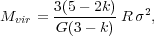
A simple and exact argument can be laid for virialized molecular clouds, that is clouds where twice the internal kinetic energy equals the potential energy. Following Solomon et al. (1987), the virial mass M_vir of a giant molecular cloud (GMC) in M is

(8)

where R is the projected radius (in pc), is the 1D velocity dispersion (in km s^-1; _3D = √3), G is the gravitational constant (G 1 / 232 M^-1 pc km² s^-2), and k is the power-law index of the spherical volume density distribution, (r) r^-k. The coefficient in front of R ² is only weakly dependent on the density profile of the virialized cloud, and corresponds to approximately 1160, 1040, and 700 for k = 0, 1, and 2 respectively (MacLaren, Richardson & Wolfendale 1988, Bertoldi & McKee 1992). Unless otherwise specified, we adopt k = 1 for the remainder of the discussion. This expression of the virial mass is fairly robust if other terms in the virial theorem (McKee & Zweibel 1992, Ballesteros-Paredes 2006), such as magnetic support, can be neglected (for a more general expression applicable to spheroidal clouds and a general density distribution see Bertoldi & McKee 1992). As long as molecular gas is dominating the mass enclosed in the cloud radius and the cloud is approximately virialized, M_vir will be a good measure of the H₂ mass.

Empirically, molecular clouds are observed to follow a size-line width relation (Larson 1981, Heyer et al. 2009) such that approximately

(9)

with C 0.7 km s^-1 pc^-0.5 (Solomon et al. 1987, Scoville et al. 1987, Roman-Duval et al. 2010). This relation is an expression of the equilibrium supersonic turbulence conditions in a highly compressible medium, and it is thought to apply under very general conditions (see Section 2.1 of McKee & Ostriker 2007 for a discussion). In fact, to within our current ability to measure these two quantities such a relation is also approximately followed by extragalactic GMCs in galaxy disks (e.g., Rubio, Lequeux & Boulanger 1993, Bolatto et al. 2008, Hughes et al. 2010).

Note that insofar as the size dependence of Eq. 9 is close to a square root, the combination of Eqs. 8 and 9 yields that M_vir ⁴, and molecular clouds that fulfill both relations have a characteristic mean surface density, _GMC, at a value related to the coefficient of Eq. 9 so that _GMC = M_vir / R² 331 C² for our chosen density profile r^-1. We return to the question of _GMC in the Milky Way in Section 4.4.

Since the CO luminosity of a cloud, L_CO, is the product of its area ( R²) and its integrated surface brightness (T_B √2 ), then L_CO = √2 ³ T_B R², where T_B is the Rayleigh-Jeans brightness temperature of the emission (see Section 1.2). Using the size-line width relation (Equation 9) to substitute for R implies that L_CO T_B ⁵. Employing this relation to replace in M_vir ⁴ we obtain a relation between M_vir and L_CO,

(10)

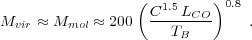
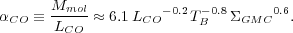
That is, for GMCs near virial equilibrium with approximately constant brightness temperature, T_B, we expect an almost linear relation between virial mass and luminosity. The numerical coefficient in Equation 10 is only a weak function of the density profile of the cloud. Then using the relation between C and _GMC we obtain the following expression for the conversion factor

(11)

Equations 10 and 11 rest on a number of assumptions. We assume 1) virialized clouds with, 2) masses dominated by H₂ that 3) follow the size-line width relation and 4) have approximately constant temperature. Equation 11 applies to a single, spatially resolved cloud, as _GMC is the resolved surface density.

We defer the discussion of the applicability of the virial theorem to Section 4.1.1, and the effect of other mass components to Section 2.3. The assumption of a size-line width relation relies on our understanding of the properties of turbulence in the interstellar medium. The result √R follows our expectations for a highly compressible turbulent flow, with a turbulence injection scale at least comparable to GMC sizes. The existence of a narrow range of proportionality coefficients, corresponding to a small interval of GMC average surface densities, is less well understood (for an alternative view on this point, see Ballesteros-Paredes et al. 2011). In fact, this narrow range could be an artifact of the small dynamic range of the samples (Heyer et al. 2009). Based on observations of the Galactic center (Oka et al. 2001) and starburst galaxies (e.g., Rosolowsky & Blitz 2005), _GMC likely does vary with environment. Equation 11 implies that any such systematic changes in _GMC will also lead to systematic changes in X_CO, though in actual starburst environments the picture is more complex than implied by Equation 11. Section 7 reviews the case of bright, dense starbursts in detail.

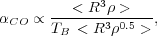
This calculation also implies a dependence of X_CO on the physical conditions in the GMC, density and temperature. Combining Eqs. 8 and 9 with M_vir R³, where is the gas density, yields ^-0.5. Meanwhile, because CO emission is optically thick the observed luminosity depends on the brightness temperature, T_B, as well as the line width, so that L_CO T_B. Substituting in the relationship between density and line width,

(12)

The brightness temperature, T_B, will depend on the excitation of the gas (Eq. 6) and the filling fraction of emission in the telescope beam, f_b. For high density and optical depth the excitation temperature will approach the kinetic temperature. Under those conditions, Eq. 12 also implies _CO ^0.5 (f_b T_kin)^-1.

Thus, even for virialized GMCs we expect that the CO-to-H₂ conversion factor will depend on environmental parameters such as gas density and temperature. To some degree, these dependencies may offset each other. If denser clouds have higher star formation activity and are consequently warmer, the opposite effects of and T_B in Eq. 12 may partially cancel yielding a conversion factor that is closer to a constant than we might otherwise expect.

We also note that relation between mass and luminosity expressed by Eq. 10 is not exactly linear, which is the reason for the weak dependence of _CO on L_CO or M_mol in Eq. 11. As a consequence, even for GMCs that obey this simple picture, _CO will depend (weakly) on the mass of the cloud considered, varying by a factor of ~ 4 over 3 orders of magnitude in cloud mass.

2.2. Galaxies

This simple picture for how the CO luminosity can be used to estimate masses of individual virialized clouds is not immediately applicable to entire galaxies. An argument along similar lines, however, can be laid out to suggest that under certain conditions there should be an approximate proportionality between the integrated CO luminosity of entire galaxies and their molecular mass. This is known as the "mist" model, for reasons that will become clear in a few paragraphs. Following Dickman, Snell & Schloerb (1986), the luminosity due to an ensemble of non-overlapping CO emitting clouds is L_{CO i} a_i T_B(a_i) _i, where a_i is the area subtended by cloud i, and T_B(a_i) and _i are its brightness temperature and velocity dispersion, respectively. Under the assumption that the brightness temperature is mostly independent of cloud size, and that there is a well-defined mean, T_B, then T_B(a_i) T_B. We can rewrite the luminosity of the cloud ensemble as L_CO √2 T_B N_clouds < R_i² (R_i)>, where the brackets indicate expectation value, N_clouds is the number of clouds within the beam, and we have used a_i = R_i². Similarly, the total mass of gas inside the beam is M_mol N_clouds < 4 / 3 R_i³ (R_i)>, where (R_i) is the volume density of a cloud of radius R_i. Using our definition from Eq. 2 and dropping the i indices, it is then clear that

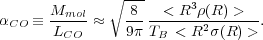(13)

If the individual clouds are virialized they will follow Eq. 8, or equivalently = 0.0635 R√. Substituting into Eq. 13 we find

(14)

which is analogous to Eq. 12 (obtained for individual clouds). As Dickman, Snell & Schloerb (1986) discuss, it is possible to generalize this result if the clouds in a galaxy follow a size-line width relation and they have a known distribution of sizes. Assuming individually virialized clouds, and using the size-line width relation (Eq. 9), we can write down Eq. 13 as

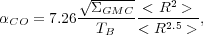(15)

where we have introduced the explicit dependence of the coefficient of the size-line width relation on the cloud surface density, _GMC. This equation is the analogue of Eq. 11.

In the context of these calculations, CO works as a molecular mass tracer in galaxies because its intensity is proportional to the number of clouds in the beam, and because through virial equilibrium the contribution from each cloud to the total luminosity is approximately proportional to its mass, as discussed for individual GMCs. This is the essence of the "mist" model: although each particle (cloud) is optically thick, the ensemble acts optically thin as long as the number density of particles is low enough to avoid shadowing each other in spatial-spectral space.

Besides the critical assumption of non-overlapping clouds, which could be violated in environments of very high density leading to "optical depth" problems that may render CO underluminous, the other key assumption in this model is the virialization of individual clouds, already discussed for GMCs in the Milky Way. The applicability of a uniform value of _CO across galaxies relies on three assumptions that should be evident in Eq. 15: a similar value for _GMC, similar brightness temperatures for the CO emitting gas, and a similar distribution of GMC sizes that determines the ratio of the expectation values <R²> / <R^2.5>. Very little is known currently on the distribution of GMC sizes outside the Local Group (Blitz et al. 2007, Fukui & Kawamura 2010), and although this is a potential source of uncertainty in practical terms this ratio is unlikely to be the dominant source of galaxy-to-galaxy variation in _CO.

2.3. Other Sources of Velocity Dispersion

Because CO is optically thick, a crucial determinant of its luminosity is the velocity dispersion of the gas, . In our discussion for individual GMCs and ensembles of GMCs in galaxies we have assumed that is ultimately determined by the sizes (through the size-line width relation) and virial masses of the clouds. It is especially interesting to explore what happens when the velocity dispersion of the CO emission is related to an underlying mass distribution that includes other components besides molecular gas. Following the reasoning by Downes, Solomon & Radford (1993) (see also Maloney & Black 1988, Downes & Solomon 1998) and the discussion in Section 2.1, we can write a cloud luminosity L_CO for a fixed T_B as L_CO^* = L_CO ^* / , where the asterisk indicates quantities where the velocity dispersion of the gas is increased by other mass components, such as stars. Assuming that both the molecular gas and the total velocity dispersion follow the virial velocity dispersion due to a uniform distribution of mass, = √GM / 5R, then L_CO^* = L_CO √M^* / M_mol, where M^* represents the total mass within radius R. Substituting L_CO = M_mol / _CO yields the result _CO L_CO^* = √M_mol M^*.

Therefore, the straightforward application of _CO to the observed luminosity L_CO^* will yield an overestimate of the molecular gas mass, which in this simple reasoning will be the harmonic mean of the real molecular mass and the total enclosed mass. If the observed velocity dispersion is more closely related to the circular velocity, as may be in the center of a galaxy, then ^* √GM^* / R and the result of applying _CO to L_CO^* will be an even larger overestimate of M_mol. The appropriate value of the CO-to-H₂ conversion factor to apply under these circumstances in order to correctly estimate the molecular mass is

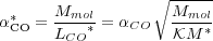(16)

where is a geometrical correction factor accounting for the differences in the distributions of the gas and the total mass, so that (^* / )². In the extreme case of a uniform distribution of gas responding to the potential of a rotating disk of stars in a galaxy center, ~ 5. Everything else being equal, in a case where M^* ~ 10 M_mol the straight application of a standard _CO in a galaxy center may lead to overestimating M_mol by a factor of ~ 7.

Note that for this correction to apply the emission has to be optically thick throughout the medium. Otherwise any increase in line width is compensated by a decrease in brightness, keeping the luminosity constant. Thus this effect is only likely to manifest itself in regions that are already rich in molecular gas. Furthermore, it is possible to show that an ensemble of virialized clouds that experience cloud-cloud shadowing cannot explain a lower X_CO, simply because there is a maximum attainable luminosity. Therefore we expect X_CO to drop in regions where the CO emission is extended throughout the medium, and not confined to collections of individual self-gravitating molecular clouds. This situation is likely present in ultra-luminous infrared galaxies (ULIRGs), where average gas volume densities are higher than the typical density of a GMC in the Milky Way, suggesting a pervading molecular ISM (e.g., Scoville, Yun & Bryant 1997). Indeed, the reduction of X_CO in mergers and galaxy centers has been modeled in detail by Shetty et al. (2011b) and Narayanan et al. (2011, 2012), and directly observed (Section 5.2, Section 5.3, Section 7.1, Section 7.2)

2.4. Optically Thin Limit

Although commonly the emission from ¹²CO J = 1 → 0 transition is optically thick, under conditions such as highly turbulent gas motions or otherwise large velocity dispersions (for example stellar outflows and perhaps also galaxy winds) then emission may turn optically thin. Thus it is valuable to consider the optically thin limit on the value of the CO-to-H₂ conversion factor. Using Eq. 5, the definition of optically thin emission (I_J = _J [B_J(T_ex) - B_J(T_cmb)], where B_J is the Planck function at the frequency _J of the J → J - 1 transition, T_ex is the excitation temperature, and T_cmb is the temperature of the Cosmic Microwave Background), and the definition of antenna temperature T_J, I_J = (2 k _J² / c²) T_J, the integrated intensity of the J → J - 1 transition can be written as

(17)

The factor f_cmb accounts for the effect of the Cosmic Microwave Background on the measured intensity, f_cmb = 1 - (e^{h _J / k T_ex} - 1) / (e^{h _J / k T_cmb} - 1). Note that f_cmb ~ 1 for T_ex ≫ T_cmb.

The column density of H₂ associated with this integrated intensity is simply N(H₂) = 1 / Z_{CO J = 0}^∞ N_J, where Z_CO is the CO abundance relative to molecular hydrogen, Z_CO = CO / H₂. For a Milky Way gas phase carbon abundance, and assuming all gas-phase carbon is locked in CO molecules, Z_CO 3.2 × 10^-4 (Sofia et al. 2004). Note, however, that what matters is the integrated Z_CO along a line-of-sight, and CO may become optically thick well before this abundance is reached (for example, Fig. 1). Indeed, Sheffer et al. (2008) analyze Z_CO in Milky Way lines-of-sight, finding a steep Z_CO 4.7 × 10^-6 (N(H₂) / 10²¹ cm^-2)^2.07 for N(H₂) > 2.5 × 10²⁰ cm^-2, with an order of magnitude scatter (see also Sonnentrucker et al. 2007).

When observations in only a couple of transitions are available, it is useful to assume local thermodynamic equilibrium applies (LTE) and the system is described by a Boltzmann distribution with a single temperature. In that case the column density will be N(CO) = Q(T_ex) e^{E₁ / k T_ex} N₁ / g₁, where E₁ is the energy of the J = 1 state (E₁ / k 5.53 K for CO), and Q(T_ex) = _{J = 0}^∞ g_J e^{-E_J / kT_ex} corresponds to the partition function at temperature T_ex which can be approximated as Q(T_ex) ~ 2 k T_ex / E₁ for rotational transitions when T_ex ≫ 5.5 K (Penzias 1975 note this is accurate to ~ 10% even down 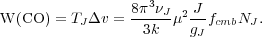to T_ex ~ 8 K). Using Eq. 17 we can then write

(18)

Consequently, adopting Z_CO = 10^-4 and using a representative T_ex = 30 K, we obtain

(19)

or _CO 0.34 M (K km s^-1 pc²)^-1. These are an order of magnitude smaller than the typical values of X_CO and _CO in the Milky Way disk, as we will discuss in Section 4. Note that they are approximately linearly dependent on the assumed Z_CO and T_ex (for T_ex ≫ 5.53 K). For a similar calculation that also includes an expression for non-LTE, see Papadopoulos et al. (2012).

2.5. Insights from Cloud Models

A key ingredient in further understanding X_CO in molecular clouds is the structure of molecular clouds themselves, which plays an important role in the radiative transfer. This is important both for the photodissociating and heating ultraviolet radiation, and for the emergent intensity of the optically thick CO lines.

The CO J = 1 → 0 transition arises well within the photodissociation region (PDR) in clouds associated with massive star formation, or even illuminated by the general diffuse interstellar radiation field (Maloney & Black 1988, Wolfire, Hollenbach & Tielens 1993). At those depths gas heating is dominated by the grain photoelectric effect whereby stellar far-ultraviolet photons are absorbed by dust grains and eject a hot electron into the gas. The main parameter governing grain photoelectric heating is the ratio T_kin^0.5 / n_e, where is a measure of the far-ultraviolet field strength, and n_e is the electron density. This process will produce hotter gas and higher excitation in starburst galaxies. At the high densities of extreme starbursts, the gas temperature and CO excitation may also be enhanced by collisional coupling between gas and warm dust grains.

Early efforts to model the CO excitation and luminosity in molecular clouds using a large velocity gradient model were carried out by Goldreich & Kwan (1974). The CO luminosity-gas mass relation was investigated by Kutner & Leung (1985) using microturbulent models, and by Wolfire, Hollenbach & Tielens (1993) using both microturbulent and macroturbulent models. In microturbulent models the gas has a (supersonic) isotropic turbulent velocity field with scales smaller than the photon mean free path. In the macroturbulent case the scale size of the turbulence is much larger than the photon mean free path, and the emission arises from separate Doppler shifted emitting elements. Microturbulent models produce a wide range of CO J = 1 → 0 profile shapes, including centrally peaked, flat topped, and severely centrally self-reversed, while most observed line profiles are centrally peaked. Macroturbulent models, on the other hand, only produce centrally peaked profiles if there are a sufficient number of "clumps" within the beam with densities n 10³ cm^-3 in order to provide the peak brightness temperature. Falgarone et al. (1994) demonstrated that a turbulent velocity field can produce both peaked and smooth line profiles, much closer to observations than macroturbulent models.

Wolfire, Hollenbach & Tielens (1993) use PDR models in which the chemistry and thermal balance was calculated self-consistently as a function of depth into the cloud. The microturbulent PDR models are very successful in matching and predicting the intensity of low-J CO lines and the emission from many other atomic and molecular species (Hollenbach & Tielens 1997, Hollenbach & Tielens 1999). For example, the nearly constant ratio of [CII] / CO J = 1 → 0 observed in both Galactic and extragalactic sources (Crawford et al. 1985, Stacey et al. 1991) was first explained by PDR models as arising from high density (n 10³ cm^-3) and high UV field ( 10³) sources in which both the [CII] and CO are emitted from the same PDR regions in molecular cloud surfaces. These models show that the dependence on CO luminosity with incident radiation field is weak. This is because as the field increases the _CO = 1 surface is driven deeper into the cloud where the dominant heating process, grain photoelectric heating, is weaker. Thus the dissociation of CO in higher fields regulates the temperature where _CO = 1.

PDR models have the advantage that they calculate the thermal and chemical structure in great detail, so that the gas temperature is determined where the CO line becomes optically thick. We note however, that although model gas temperatures for the CO J = 1 → 0 line are consistent with observations the model temperatures are typically too cool to match the observed high-J CO line emission (e.g., Habart et al. 2010). The model density structure is generally simple (constant density or constant pressure), and the velocity is generally considered to be a constant based on a single microturbulent velocity. More recent dynamical models have started to combine chemical and thermal calculations with full hydrodynamic simulations.