Annu. Rev. Astron. Astrophys. 2013. 51: 207-268 Copyright © 2013 by Annual Reviews. All rights reserved

1. INTRODUCTION

Molecular hydrogen, H₂, is the most abundant molecule in the universe. With the possible exception of the very first generations of stars, star formation is fueled by molecular gas. Consequently, H₂ plays a central role in the evolution of galaxies and stellar systems (see the recent review by Kennicutt & Evans 2012). Unfortunately for astronomers interested in the study of the molecular interstellar medium (ISM), cold H₂ is not directly observable in emission. H₂ is a diatomic molecule with identical nucleii and therefore possesses no permanent dipole moment and no corresponding dipolar rotational transitions. The lowest energy transitions of H₂ are its purely rotational quadrupole transitions in the far infrared at = 28.22 µm and shorter wavelengths. These are weak owing to their long spontaneous decay lifetimes _decay ~ 100 years. More importantly, the two lowest para and ortho transitions have upper level energies E / k 510 K and 1015 K above ground (Dabrowski 1984). They are thus only excited in gas with T 100 K. The lowest vibrational transition of H₂ is even more difficult to excite, with a wavelength = 2.22 µm and a corresponding energy E / k = 6471 K. Thus the cold molecular hydrogen that makes up most of the molecular ISM in galaxies is, for all practical purposes, invisible in emission.

Fortunately, molecular gas is not pure H₂. Helium, being monoatomic, suffers from similar observability problems in cold clouds, but the molecular ISM also contains heavier elements at the level of a few × 10^-4 per H nucleon. The most abundant of these are oxygen and carbon, which combine to form CO under the conditions prevalent in molecular clouds. CO has a weak permanent dipole moment (µ 0.11 D = 0.11 × 10^-18 esu cm) and a ground rotational transition with a low excitation energy h / k 5.53 K. With this low energy and critical density (further reduced by radiative trapping due to its high optical depth), CO is easily excited even in cold molecular clouds. At a wavelength of 2.6 mm, the J = 1 → 0 transition of CO falls in a fairly transparent atmospheric window. It has thus become the workhorse tracer of the bulk distribution of H₂ in our Galaxy and beyond.

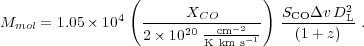
As a consequence, astronomers frequently employ CO emission to measure molecular gas masses. The standard methodology posits a simple relationship between the observed CO intensity and the column density of molecular gas, such that

(1)

where the column density, N(H₂), is in cm^-2 and the integrated line intensity, W(CO) ¹, is in traditional radio astronomy observational units of K km s^-1. A corollary of this relation arises from integrating over the emitting area and correcting by the mass contribution of heavier elements mixed in with the molecular gas,

(2)

Here M_mol has units of M and L_CO is usually expressed in K km s^-1 pc². L_CO relates to the observed integrated flux density in galaxies via L_CO = 2453 S_CO v D_L² / (1 + z), where S_CO v is the integrated line flux density, in Jy km s^-1, D_L is the luminosity distance to the source in Mpc, and z is the redshift (e.g., Solomon & Vanden Bout 2005, use Eq. 7 to convert between W(CO) and S_CO v). Thus _CO is simply a mass-to-light ratio. The correction for the contribution of heavy elements by mass reflects chiefly helium and amounts to a 36% correction based on cosmological abundances.

Both X_CO and _CO are referred to as the "CO-to-H₂ conversion factor." For X_CO = 2 × 10²⁰ cm^-2(K km s^-1)^-1 the corresponding _CO is 4.3 M (K km s^-1 pc²)^-1. To translate integrated flux density directly to molecular mass, Equation 2 can be written as

(3)

For convenience we define

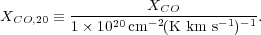(4)

We discuss the theoretical underpinnings of these equations in Section 2.

Note that the emission from CO J = 1 → 0 is found to be consistently optically thick except along very low column density lines-of-sight, as indicated by ratios of ¹²CO to ¹³CO intensities much lower than the isotopic ratio. The reason for this is simple to illustrate. The optical depth of a CO rotational transition is

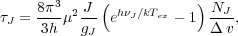(5)

where J and N_J are the rotational quantum number and the column density in the upper level of the J → J - 1 transition, is the frequency, T_ex is the excitation temperature (in general a function of J, and restricted to be between the gas kinetic temperature and that of the Cosmic Microwave Background), v is the velocity width, µ is the dipole moment, g_J = 2J + 1 is the statistical weight of level J, and h and k are the Planck and Boltzmann constants respectively. Under typical conditions at the molecular boundary, 1 for the J = 1 → 0 transition requires N(H₂) 2-3 × 10²⁰ cm^-2 for a Galactic carbon gas-phase abundance A_C ~ 1.6 × 10^-4 (Sofia et al. 2004). At the outer edge of a cloud the carbon is mainly C⁺, which then recombines with electrons to form neutral C (Fig. 1). Carbon is converted to CO by a series of reactions initiated by the cosmic-ray ionization of H or H₂ (e.g., van Dishoeck & Black 1988) and becomes the dominant carrier of carbon at A_V ~ 1-2. The CO J = 1 → 0 line turns optically thick very quickly after CO becomes a significant carbon reservoir, over a region of thickness A_V ~ 0.2-0.3 for a typical Galactic dust-to-gas ratio (c.f., Eq. 21).

Figure 1. Calculated cloud structure as a function of optical depth into the cloud. Top panel shows the fractional abundance of HI, H2, C+, C, and CO. Middle panel shows their integrated column densities from the cloud edge. Bottom panel shows the emergent line intensity in units of K km s-1 for [CII] 158 µm, [CI] 609 µm, and CO J = 1 → 0. The grey vertical bar shows where CO J = 1 → 0 becomes optically thick. At the outer edge of the cloud gas is mainly HI. H2 forms at AV ~ 0.5 while the carbon is mainly C+. The C+ is converted to C at AV ~ 1 and CO dominates at AV 2. The model uses constant H density n = 3 × 103 cm-3, a radiation field = 30 times the interstellar radiation field of Draine (1978), a primary cosmic-ray ionization rate of 2× 10-16 s-1 per hydrogen nucleon, and are based on the PDR models of Wolfire, Hollenbach & McKee (2010) and Hollenbach et al. (2012).

Equations 1 and 2 represent highly idealized, simplified relations where all the effects of environment, geometry, excitation, and dynamics are subsumed into the X_CO or _CO coefficients. A particular example is the effect that spatial scales have on the CO-to-H₂ conversion factor. Indeed, for the reasons discussed in the previous paragraph, X_CO along a line-of-sight through a dense molecular cloud where A_V 10 is not expected to be the same as X_CO along a diffuse line-of-sight sampling mostly material where A_V < 1 (see, for example, Pineda et al. 2010, Liszt & Pety 2012). Thus on small spatial scales we expect to see a large variability in the CO-to-H₂ conversion factor. This variability will average out on the large spatial scales, to a typical value corresponding to the dominant environment. Because of the large optical depth of the CO J = 1 → 0 transition the velocity dispersion giving rise to the width of the CO line will also play an important role on W(CO), and indirectly on X_CO. Indeed, there is not one value of X_CO that is correct and applicable to each and every situation, although there are values with reasonable uncertainties that are applicable over large galactic scales.

The plan of this work is as follows: in the remainder of this section we provide a brief historical introduction. In Section 2 we present the theoretical background to the CO-to-H₂ conversion factor. In Section 4 we review the methodology and measurements of X_CO in the Milky Way, the best understood environment. We characterize the range of values found and the underlying physics for each measurement technique. In Section 5 we review the literature on X_CO determinations in "normal" star-forming galaxies and discuss the techniques available to estimate X_CO in extragalactic systems. In Section 6 we consider the effect of metallicity, a key local physical parameter. In Section 7 we review the measurements and the physical mechanisms affecting the value of the CO-to-H₂ conversion factor in the starburst environments of luminous and ultraluminous galaxies. In Section 8 we consider the explicit case of X_CO in high redshift systems, where a much more restricted range of observations exist. In Section 3 we discuss the results of recent calculations of molecular clouds including the effects of turbulence and chemistry. Finally, in Section 9 we will offer some recommendations and caveats as to the best values of X_CO to use in different environments, as well as some suggestions about open avenues of research on the topic.

1.1. Brief Historical Perspective

Carbon monoxide was one of the first interstellar medium molecules observed at millimeter wavelengths. Wilson, Jefferts & Penzias (1970) reported the discovery of intense CO emission from the Orion nebula using the 36 foot NRAO antenna at Kitt Peak, Arizona. Surveys of molecular clouds in the Galaxy (e.g., Solomon et al. 1972, Wilson et al. 1974, Scoville & Solomon 1975, Burton et al. 1975) established molecular gas to be widespread in the inner Milky Way with a distribution that resembles giant HII regions more closely than that of atomic hydrogen gas. The combination of CO and -ray observations demonstrated that H₂ dominates over HI by mass in the inner Galaxy (Stecker et al. 1975). By the end of the following decade, these studies extended to complete the mapping of the Galactic plane (Dame et al. 1987).

The first extragalactic detections of CO occurred in parallel with these early Galactic surveys (Rickard et al. 1975, Solomon & de Zafra 1975). They found CO to be particularly bright in galaxies with nuclear activity such as M 82 and NGC 253. The number of extragalactic CO observations grew rapidly to include several hundred galaxies over the next two decades (Young & Scoville 1991, Young et al. 1995), and CO emission was employed to determine galaxy molecular masses (Young & Scoville 1982). By the late 1980s, the first millimeter interferometers spatially resolved molecular clouds in other galaxies (Vogel, Boulanger & Ball 1987, Wilson et al. 1988). Such observations remain challenging, though powerful new interferometric facilities such as the Atacama Large Millimeter Array (ALMA) will change that.

The first detection of CO at cosmological redshifts targeted ultraluminous infrared sources and revealed very large reservoirs of highly excited molecular gas (Brown & Vanden Bout 1991, Solomon, Downes & Radford 1992). Because of the deep integrations required, the number of high redshift CO detections grew slowly at first (Solomon & Vanden Bout 2005), but this field is now developing rapidly driven by recent improvements in telescope sensitivity (see the review by Carilli & Walter in this issue). An increased appreciation of the roles of gas and star formation in the field of galaxy evolution and the according need to determine accurate gas masses provides one of the motivations for this review.

1.2. CO Excitation

Under average molecular cloud conditions, CO molecules are excited through a combination of collisions with H₂ and radiative trapping. They de-excite through spontaneous emission and collisions, except at very high densities where collisions are extremely frequent. Neglecting the effect of radiative trapping, radiative and collisional de-excitation will balance for a critical density n_cr,J A_J / _J(T_kin) (neglecting the effects of stimulated emission), where T_kin is the kinetic gas temperature. Thus, for n≫ n_cr,J and excitation temperatures T_ex,J ≫ E_J / k 5.53 J (J + 1) / 2 K the upper level of the J → J - 1 transition will be populated and the molecule will emit brightly. In these expressions A_J is the Einstein coefficient for spontaneous emission (only transitions with | J| = 1 are allowed), A_J = 64 ⁴ _J³ µ² J / (3 h c³ g_J) (A₁ 7.11 × 10^-8 s^-1). The parameter _J(T) is the corresponding collisional coefficient (the sum of all collisional rate coefficients for transitions with upper level J), which is a weak function of temperature. For CO, ₁ ~ 3.26 × 10^-11 cm³ s^-1 for collisions with H₂ at T_kin 30 K (Yang et al. 2010). T_ex,J refers to the excitation temperature, defined as the temperature needed to recover the relative populations of the J and J-1 levels from the Boltzmann distribution. In general, T_{ex, J} will be different for different transitions.

The critical density for the CO J = 1 → 0 transition is n(H₂)_cr,1 ~ 2200 cm^-3. Higher transitions require rapidly increasing densities and temperatures to be excited, as n_cr,J J³ and E_J J². The high optical depth of the CO emission relaxes these density requirements, as radiative trapping reduces the effective density required for excitation by a factor ~ 1 / _J (the precise factor corresponds to an escape probability and is dependent on geometry).

The Rayleigh-Jeans brightness temperature, T_J, measured by a radio telescope for the J → J - 1 transition will be

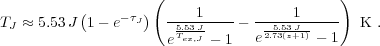(6)

The final term accounts for the effect of the Cosmic Microwave Background at the redshift, z, of interest. Note that frequently the Rayleigh-Jeans brightness temperature is referred to as the radiation temperature. Observations with single-dish telescopes usually yield antenna temperatures corrected by atmospheric attenuation (T_A^*), or main beam temperatures (T_MB), such that T_MB = _MB T_A^* where _MB is the main beam efficiency of the telescope at the frequency of the observation (see Kutner & Ulich 1981 for further discussion). The Rayleigh-Jeans brightness temperature T_J is identical to T_MB for compact sources, while extended sources may couple to the antenna with a slightly different efficiency.

Extragalactic results, and measurements with interferometers, are frequently reported as flux densities rather than brightness temperatures. The relations between flux density (in Jy) and Rayleigh-Jeans brightness temperature (in K) in general, and for CO lines, are

(7)

where is the half-maximum at full width of the telescope beam (in arcsec), and is the wavelength of a transition (in mm).

The Rayleigh-Jeans brightness temperature, T_J, excitation temperature, T_ex,J, and kinetic temperature, T_kin, are distinct but related. The ¹²CO transitions usually have _J ≫ 1, making the Rayleigh-Jeans brightness temperature a probe of the excitation temperature, T_J ~ T_ex,J for T_ex,J ≫ 5.53 J K. In general T_ex,J can be shown to be in the range T_cmb ≤ T_ex,J ≤ T_kin. At densities much higher than n_cr,J the population of the levels J and lower will approach a Boltzmann distribution, and become "thermalized" at the gas kinetic temperature, T_ex,J T_kin. The corresponding Rayleigh-Jeans brightness can be computed using Eq. 6. When T_ex,J < T_kin, usually T_ex,J / T_ex,J-1 < 1 for lines arising in the same parcel of gas, and the excitation of the J level is "subthermal" (note that this is not equivalent to T_J / T_J-1 < 1, as is sometimes used in the literature).

¹ Henceforth we refer to the most common ¹²C¹⁶O isotopologue as simply CO, and unless otherwise noted to the ground rotational transition J = 1 → 0. Back.