1.3. FLUCTUATIONS

In previous sections we investigated the orbits of stars in a smooth, time-independent model of the galaxy's gravitational potential. In reality the potential contains time-dependent features and in this section we investigate how these features drive evolution.

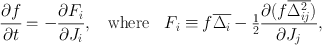
A fundamental result is obtained by multiplying the equation of motion ṗ = −∇Φ by p and rearranging the result to

(1.42)

Thus stars change their energies if and only if the potential is time-dependent. Fluctuations in the potential enable stars to exchange energy.

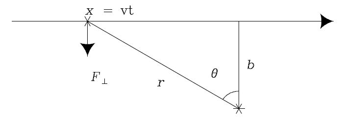Figure 1.11. A fast encounter between two stars at speed v and impact parameter b. The force perpendicular to the relative velocity is ∼ Gm1m2 / b2 and it acts for a time ∼ 2b / t.

1.3.1. Two-body scattering

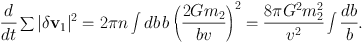
The most obvious source of fluctuations is the moving gravitational potentials of individual stars. When stars of mass m₁ and m₂ pass each other at speed v and impact parameter b (Fig. 1.11) the effect is an exchange of momentum along the line that is perpendicular to the mutual velocity and has magnitude ∼ 2Gm₁m₂ / bv. So the encounter adds to the velocity of m₁ a velocity δ v₁ of magnitude ∼ 2Gm₂ / bv. The direction of these increments is random, so we add them in quadrature. The rate of such encounters is ∼ 2π nv bd b, where n is the number density of stars, so the rate of change of ∑|δ v₁|² is

(1.43)

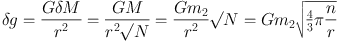
The integral diverges at both ends of the range of integration. The divergence at small b is an artifact that can be traced to our use of 2Gm₂ / bv as the magnitude of the velocity change in an encounter: an accurate calculation shows that the velocity change never exceeds v (Binney & Tremaine, 2008, eq. 3.53a). The divergence at large b is real, and indicates that encounters with impact parameters that are on the order of the size of the system dominate. Physically, what this means is that the dominant source of fluctuations is Poisson fluctuations in the number of stars in substantial parts of the system. The mass inside a volume of radius r will fluctuate by δ M ∼ M / √N, where N = 4 / 3π r³n is the number of stars in this volume. Just outside this volume the gravitational field will fluctuate by

(1.44)

This fluctuation acts for a time ∼ r / v so it changes the velocity of any star by

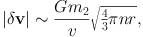(1.45)

which grows with r, thus confirming that large-scale fluctuations are the most effective. If we accept that the dominant fluctuations are those involving half the system, so r is about half the system size R, we conclude that the number of half-crossing times r / v required to change v by of order itself is

(1.46)

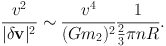
The virial theorem implies that v² ≃ GM / R, so

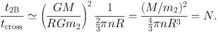(1.47)

For a galaxy this number of half-crossing times is many times the age of the Universe, so the fluctuations associated with the motions of individual stars are unimportant. But for a globular cluster, which has N ≲ 10⁵, R ∼ 3 pc and v ∼ 6 km sec⁻¹ so r / v ∼ 0.25 Myr, v changes by order itself in ∼ 6 Gyr so the process is significant. In an open cluster the process is even more important.

Two-body interactions randomise the distribution of stars in phase space and thus drive the system towards thermal equilibrium. No such equilibrium is possible for a stellar system that is only confined by its own gravity (Binney & Tremaine, 2008, §4.10). But we can understand the impact of two-body interactions by considering the consequences of trying to reach thermal equilibrium.

The speed v_e required to escape from a stellar system is never much larger than the system's characteristic velocity dispersion σ – one can easily show from the virial theorem that the mass-weighted rms of the local escape speed is only twice the mass-weighted rms velocity dispersion: ⟨ v_e²⟩^1/2 = 2 ⟨σ²⟩^1/2. Consequently, the velocity distribution is always distinctly non-Gaussian. Two-body scattering drives the velocity distribution towards Gaussianity, so it is constantly trying to repopulate the missing tail of the velocity distribution at v ≳ 2σ. Stars scattered into this domain are free and leave the system, to the system loses mass by evaporation on the two-body timescale.

In thermal equilibrium there would be equipartition between the particles. So massive stars would have a smaller velocity dispersion than low-mass stars. Consequently, two-body interactions are constantly transferring energy from more massive to less massive stars, with the consequence that the massive stars sink towards the centre of the system: two-body scattering drives mass segregation.

In thermal equilibrium all parts of a body have the same temperature. In a self-gravitating system there is a tendency for the centre to be hotter than the outside, if only because the escape speed decreases outwards. So two-body interactions tend to transfer energy outwards from the core to the envelope. By the virial theorem, a self-gravitating system that loses energy contracts and gets hotter, while one that gains energy expands and becomes cooler. So the conduction of heat from the core to the envelope increases the difference in temperature between the two parts of the system and accelerates the heat flow. The upshot is the gravithermal catastrophe in which the core contracts in both size and mass until it contains only a few stars.

The point to note about evaporation, mass-segregation and the gravithermal catastrophe is they are all consequences of fluctuations in the gravitational field driving the system towards an unattainable thermal equilibrium. In star clusters fluctuations associated with individual stars are sufficient to generate these effects on astronomically interesting timescales. In galaxies they are not, but evaporation and the gravithermal catastrophe will be driven by whatever fluctuations do occur, while equipartition won't be because it depends on stars of different masses experiencing different fluctuations. Sources of significant fluctuations in galaxies include giant molecular clouds, spiral arms, satellite galaxies, and high-speed encounters with other comparable galaxies.

1.3.2. Orbit-averaged Fokker-Planck equation

In this section we develop a general framework for handling the impact of fluctuations. The general idea is that, by the strong Jeans theorem (§ 1.1.2) the galaxy's distribution function is at all times a function f(J, t) of the actions. Fluctuations (and resonances) cause this function to evolve by causing innumerable small changes δJ in the actions of individual stars. Let P(J, Δ) d³ Δ δ t be the probability that in time δ t a star with actions J is scattered to the action-space volume d³ Δ centred on J + Δ. The number of stars in the action-space volume d³ J is (2π)³ f(J, t) d³ J, so the number of stars leaving this volume in δ t is

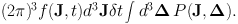(1.48)

Similarly, the number of stars that are scattered into this volume is

(1.49)

Hence the rate of change of the distribution function is

(1.50)

Since scattering events change actions only slightly, P(J, Δ) is appreciable only for |Δ| ≪ |J|. So we can truncate after just a few terms the Taylor series expansion in J of the product f(J, t) P(J, Δ):

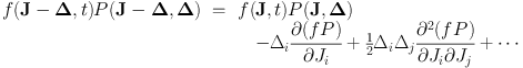(1.51)

Substituting the first three terms on the right side of this expression into equation (1.50) and cancelling terms, we obtain

(1.52)

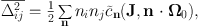
(1.53)

Equation (1.52) is the orbit-averaged Fokker-Planck equation. It states that the rate of change of the distribution function is minus the divergence of the flux F of stars in action space, and we have an expression for that flux in terms of the diffusion coefficients defined by equations (1.53). The latter are simply the expectation value and the variance of the probability distribution of changes in actions per unit time.

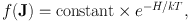
The diffusion coefficients reflect the physics of whatever is responsible for causing the fluctuations. In some circumstances, for example in a star cluster, the fluctuations will be approximately thermal in nature, with temperature T. Then the principle of detailed balance requires that the stellar flux vanish when the objects being scattered are in thermal equilibrium with the fluctuations. That is, F = 0 for

(1.54)

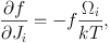
where H(J) is the Hamiltonian. In this case we have

(1.55)

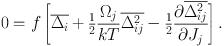
so F = 0 implies that

(1.56)

Clearly the square bracket must vanish, so we obtain an expression for the first-order diffusion coefficient in terms of the second-order coefficient (Binney & Lacey, 1988)

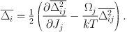(1.57)

This expression is useful because it enables us to obtain the first-order diffusion coefficients Δ_i from the second-order diffusion coefficients Δ_ij², and, while Δ_ij² can be obtained from first-order perturbation theory (see below), a direct calculation of Δ_i requires second-order perturbation theory.

The diffusion coefficients are conveniently calculated by expanding the potential in angle-action coordinates

(1.58)

where Φ₀(x) is the potential of the underlying Hamiltonian H₀(J) and Φ₁ is the fluctuating part of the potential. Hamilton's equation of motion for J is

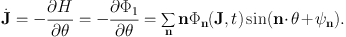(1.59)

To get a random change in J, we need to integrate this equation of motion for a time T that is longer than the auto-correlation time of the fluctuations. We do this by expanding the variables in powers of Φ₁ / Φ₀:

(1.60)

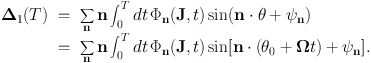(1.61)

To obtain the second-order diffusion coefficient we multiply this equation by itself and average over initial phases θ₀. After reordering the integrals so θ₀ is integrated over first, we find that the innermost integral is

(1.62)

Using 2sinA sinB = cos(A − B) − cos(A + B) and that the integral of any cosine that depends on θ₀ will vanish, we conclude that the innermost integral vanishes unless n′ = n, ¹ when it's equal to 1/2 cos[n · Ω₀(t − t′)]. Hence

(1.63)

Next we take the ensemble average over the fluctuations that are represented by Φ_n. We assume that they are a stationary random process so the autocorrelation of Φ_n(J, t) depends only on the time lag t− t′:

(1.64)

with this assumption we have

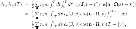(1.65)

where in the second line we have introduced new coordinates u = t + t′ and v = t − t′. Given that we want T to be bigger than the autocorrelation time of the fluctuations, we have that whenever c_n(J, v) is non-negligible, |v| ≪ T, so term in the integrand that's proportional to |v| can be neglected, leaving a result that's proportional to T. The diffusion coefficient is the coefficient of proportionality, so

(1.66)

where _n(J, ω) is the power spectrum of the fluctuations:

(1.67)

The bottom line of this result is that the ability of a star to diffuse through phase space hinges on whether the fluctuations contain power at one of the star's natural frequencies n · Ω₀. In particular, if the fluctuations are periodic in time, for example because they arise from a normal mode of the system, they will drive diffusion only of stars that resonate with them. In practice periodic fluctuations will simply depopulate narrow regions of phase space: stars for which n · Ω₀ is equal to the frequency of the fluctuation will be scattered to new actions and then cease to be resonant because fundamental frequencies are functions of the actions. Sellwood & Kahn (1991) find evidence for such action-space “grooves” in numerical simulations of stellar discs and show that they can generate new spiral features, which in their turn generate other grooves.

1.3.3. Heating of the solar neighbourhood

Fig. 1.12 shows the radial, vertical and azimuthal velocity dispersions of groups of nearby stars with accurate space velocities as a function of the colour of the stars. Blue stars are plotted on the left and red stars on the right, so all three components of velocity dispersion increase from blue to red. Blue stars are massive and short-lived, so in the blue bins all stars are quite young, while red stars live longer than the age of the galaxy, so in the red bins we have stars of all ages, but with a bias to old stars because the star-formation rate was higher in the past than it is now. So the variation of velocity dispersion with colour indicates that the random velocities of stars increase over time. From these data and isochrones one can deduce how velocity dispersion increases with age, and the conclusion is that σ ∼ t^0.35 (Aumer & Binney, 2009).

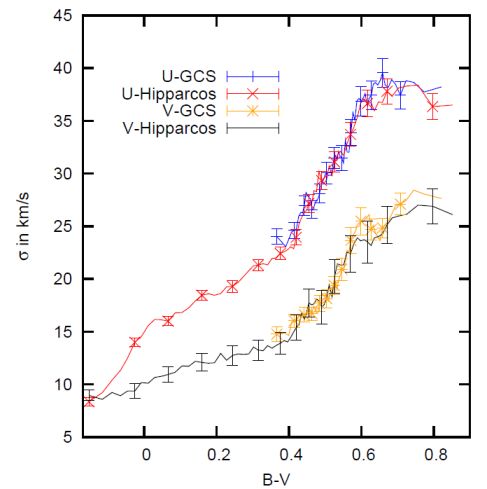Figure 1.12. The velocity dispersions of Hipparcos stars grouped by colour. From Aumer & Binney (2009).

It's instructive to infer from this result how the diffusion coefficients must scale with |J|. We make two simplifying assumptions: (i) that the dominant scatterers are much more massive than stars, and (ii) that the velocity dispersions of groups of stars scale with the mean actions in the group as

(1.68)

These relations are exact in the epicycle approximation, in which the radial and vertical oscillations of stars are harmonic, so for example J_r = E_R / κ. ² Since scattering must be dominated by giant molecular clouds and spiral arms, the assumption of massive scatterers will be a good one. In thermal equilibrium with such massive bodies, stars would have velocity dispersions that are larger than those of the clouds and arms ( ∼ 7 km sec⁻¹) by the square root of the ratio of masses, so the stars' velocity dispersion would be > 1000 km sec⁻¹. Consequently, we can use equation (1.57) in the limit of infinite temperature, ³ when the Fokker-Planck equation simplifies to

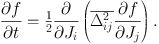(1.69)

Stars are born on orbits that have non-negligible angular momenta L_z ≡ J_φ but small values of J_r and J_z. Consequently, a young population is initially distributed in action space along the L_z axis, and diffusion of this population is predominantly away from this line, towards larger values of J_r and J_z. For this reason we neglect derivatives with respect to J_φ in equation (1.69).

In problems involving the ordinary diffusion equation, a key solution is the Green's function exp(−x² / 2t) / (2π t)^1/2, which describes the spatial distribution at time t of particles injected at x = 0 at time t = 0. Analogously, we seek a Green's function of the form

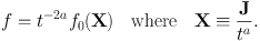(1.70)

In this solution the mean value of |J| will increase with time as t^a, and the power of t multiplying f₀ ensures that the total number of stars ∫ d L_z ∫ d J_rd J_z f is conserved as stars diffuse from the axis. Suppose Δ_ij² scales such that Δ_ij²(k J) = k^b Δ_ij²(J). Then putting k = t^−a we have Δ_ij²(x) = t^−ab Δ_ij²(J). Evaluating both sides of equation (1.69) with these assumptions yields

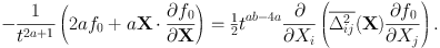(1.71)

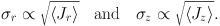
This equation can be valid at all times only if 2a + 1 = 4a − ab, so b = 2 − 1/a. Consequently, the empirical result ⟨ J_r ⟩ ∼ σ_r² ∼ t^2/3 implies a ≃ 2/3 and b ≃ 1/2.

The scaling σ_r ∼ t^1/2, which has been advocated by Wielen (1977) and several subsequent authors, implies a = b = 1. A simple argument shows that it is implausible for the diffusion coefficients to grow so rapidly with |J|. In the epicycle approximation, J_r differs from the epicycle energy E_R only by the (constant) epicycle frequency, so Δ_r ∼ Δ E_R = v · δv, where δv is the projection into the equatorial plane of the change in a star's velocity as a result of a scattering event. Hence ⟨Δ_r²⟩ ∼ |J| implies

(1.72)

That is, σ_r ∼ t^1/2 implies that |δ v| is independent of |v|. However, gravitational scattering always causes the momentum change δ v to decrease with increasing speed because the gravitational force is independent of speed and the time for which it acts decreases as 1/|v|.

Can we derive Δ_ij²(kJ) ∼ k^1/2 Δ_ij²(J) from physics? Binney & Lacey (1988) show that this scaling is predicted by the model of cloud-star scattering that was introduced by Spitzer & Scwarzschild (1953). However, this model is defective in two respects: (i) it assumes that the relative velocity with which a star encounters a cloud is dominated by epicycle motion rather than differential rotation, and, more seriously, (ii) it assumes that stars are confined to the equatorial plane. In reality as a star ages it oscillates with increasing amplitude and period perpendicular to the plane, and these oscillations decrease its probability of being scattered by a cloud. Consequently, when this effect is taken into account, Δ_ij²(J) increases with |J| more slowly than as |J|^1/2.

Binney & Lacey (1988) show that three-dimensional scattering by molecular clouds generates a tensor of diffusion coefficients Δ_ij² which is highly anisotropic. The consequence of this anisotropy is that we expect σ_z / σ_r ∼ 0.8, which is significantly larger than the observed value, ∼ 0.6. Sellwood (2008) argues that the discrepancy arises from the erroneous assumption of an isotropic distribution of encounters: as in two-body scattering, distant encounters are important, and since both stars and clouds lie within the disc, distant encounters are dominated by the velocity components that lie within the plane and do not change J_z.

Thus it seems that scattering of stars by giant molecular clouds may set the ratio of the vertical and horizontal velocity dispersions of disc stars. While star-cloud scattering makes a significant contribution to the secular increase in the velocity dispersions of stars, it probably cannot account fully for the data because its effectiveness declines rapidly with increasing velocity dispersion and thus cannot account for the numbers of stars with radial dispersions ≳ 30 km sec⁻¹.

¹ Since we are using cosine series, we need sum over only half of n space so n′ will never equal −n. Back.

² Quite generally we have that Ω_r J_r is equal to the time-averaged value of v_R² along any orbit. Back.

³ See Appendix B of Binney & Lacey (1988) for a rigorous justification of this step. Back.