1.4. SPIRAL STRUCTURE

Thin galactic discs are extremely prone to generating spiral structure. Many manifestations of spirality arise from gas-dynamics rather than stellar dynamics – for example the chains of blue stars so evident in blue and UV exposures, and the spiral distributions of H I and CO detected at radio frequencies. In such cases the old stellar disc is believed to carry a large-amplitude spiral also, but it is not easy to detect these a stellar spirals. It is most evident in near IR photometry, which is dominated by a combination of stars near the top of the giant branch and low-mass main-sequence stars (Rix & Zarisky, 1995). The former are a measure of recent star formation so they tell us more about gas than stellar dynamics, but the latter contain most of the mass of the disc, so are a window into the key dynamics. Rix & Zarisky (1995) find that the 2.2 µm surface brightnesses of spiral galaxies carry spiral structures that have amplitudes of order unity, and that the fluctuation in the surface density of stars is probably nearly as large. Radio-frequency spectral lines and the Hα line show that spiral disturbances are associated with streaming velocities ∼ 7 km sec⁻¹.

Spiral structure proves to be an intrinsically non-linear phenomenon, and as a consequence our understanding of it is still frustratingly incomplete. It's raison d'être is, however, clear: it is the principal means by which galaxies transport angular momentum outwards, which enables them to increase their entropy – i.e., heat their discs. We start our study of spiral structure by examining how this heating comes about.

1.4.1. Secular evolution driven by spiral structure

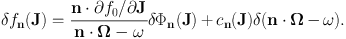
Let's assume that spiral structure is a nearly stationary pattern that rotates at some fixed angular speed Ω_p. In this case, when we write the potential of the spiral structure in angle-action variables (eq. 1.58), the expansion coefficients Φ_n(J, t) will contain only multiples of Ω_p in their temporal Fourier transforms. Hence the power spectrum of the potential c_n(J, ω), which appears in equation (1.66) for the diffusion coefficients, will be non-zero only when ω is equal to one of these frequencies, so the spiral will enable only a minority of stars to diffuse. We now examine the impact of the spiral on the minority stars that resonate with it.

If we work in the frame of reference that rotates at frequency Ω_p, the motion of each star is governed by a time-independent Hamiltonian, the numerical value of which, the Jacobi constant, is an isolating integral. In terms of the energy E of motion in the non-rotating frame, the rotating-frame Hamiltonian is

(1.73)

Since H is an integral, d H = 0 and changes in E and L_z caused by the spiral satisfy

(1.74)

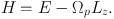
Fig. 1.13 is a plot of E versus L_z, and equation (1.74) states that in this figure a steadily rotating spiral moves stars on lines of slope Ω_p. The physically accessible region is bounded below by the locus of circular orbits, which are the orbits with the largest value of L_z for each given E, so there are no orbits in the shaded region below this boundary. The slope of the boundary, (∂ E/∂ L_z)_{Jr = 0}, is the circular frequency Ω(L_z). Clearly at the corotation resonance (CR), where Ω(L_z) = Ω_p, the spiral scatters stars from one circular orbit to another. Elsewhere, the spiral scatters stars away from the boundary, to places where the energy exceeds that of the circular orbit of the given value of L_z, and the additional energy will be invested in epicyclic motion. Inside the CR, the angular momenta of stars must be reduced, while outside the CR it must be increased. Thus the spiral must move angular momentum outwards.

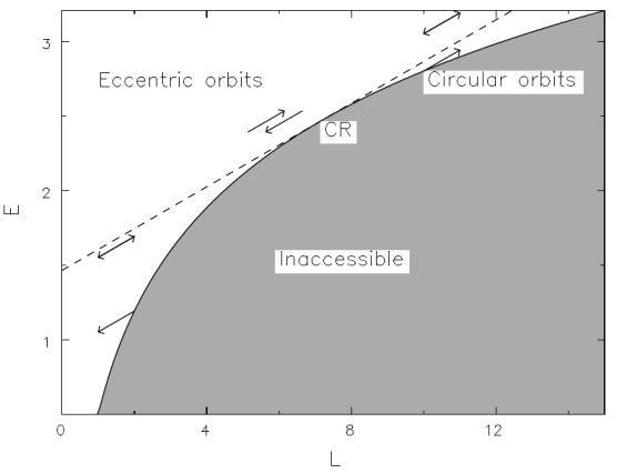Figure 1.13. Energy versus angular momentum for planar orbits in an axisymmetric potential – a “Lindblad diagram”. No orbits lie in the shaded area, which is bounded by the points of circular orbits. A potential that is stationary in a rotating frame moves stars along lines with slope d E / d Lz = Ωp. (From Sellwood & Binney 2002)

Sellwood & Binney (2002) explored these phenomena with N-body simulations of discs. In one experiment they introduced an action-space groove into the initial conditions to generate an isolated, transient spiral feature. The left panel of Fig. 1.14 shows the distribution of ensuing changes in L_z versus initial L_z. Vertical lines mark the locations of the CR and Lindblad resonances for the measured pattern speed. Stars interior to the CR gain L_z and transfer to outside the CR, while those outside the CR lose L_z and move inwards. Thus these stars swap places. The right panel explains how this is done by plotting orbits in the (φ, R) plane when a steady two-armed perturbation is imposed. There are islands formed by orbits that are trapped at the resonance, and wavy lines of orbits that continue to circulate. Orbits forming the island constantly move from inside to outside the CR and back again. When a spiral potential emerges, it creates islands which grow with the potential by sweeping up orbits from the wavy regions. When the potential fades, the islands shrink and the trapped orbits are released on each side. A star that was on an inner wavy orbit at entrapment may move on a trapped orbit from inside the CR to outside the CR before being released to a wavy orbit outside the CR. The maximum distance stars can move their guiding centres is set by the largest extent of the islands. Stars that start far inside the CR are released far outside the CR. The tendency for the populated regions in the left panel of Fig. 1.14 to slope from top left to bottom right with gradient −2 confirms this picture. Sellwood & Binney (2002) called this process of swapping places around CR churning.

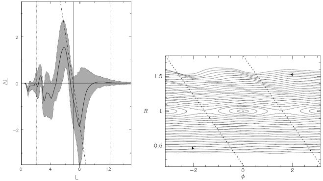Figure 1.14. Left: the distribution of changes in angular momentum amongst the first 20% of stars in an N-body simulation when they are ordered by initial epicycle energy. The vertical lines show the angular momenta corresponding to the ILR, CR and OLR of the spiral pattern within the simulation. The full curve shows the mean of the distribution and the shaded region is bounded by its 20th and 80th percentiles. The dashed line has a slope of −2. The right panel shows the response of initially circular orbits to a transient spiral potential (after Sellwood & Binney 2002).

In another experiment Sellwood & Binney allowed a disc to evolve for ∼ 5 Gyrwithout seeding any spiral structure. Irregular and quite weak spiral structure emerged as the disc was evolved. Fig. 1.15 shows histograms of the final radii of stars that all started from the narrow radial bands marked. Stars that started at the current radius of the Sun finished at radii that are often 1.2−2 kpc from R₀. From the strength of spiral structure seen in NIR photometry, Sellwood & Binney estimated that over the Hubble time stars will typically migrate ∼ 2 kpc from their birth radii.

Figure 1.15. Each panel shows the distribution of the final guiding-centre radii of the stars in a disc simulation whose initial guiding-centre radii lay within the region between the dotted vertical lines. The disc had a flat rotation curve, Q = 1.5, and half of the radial force was provided by a fixed halo. The duration of the simulation was ∼ 4 Gyr. (From Sellwood & Binney 2002).

1.4.2. Propagation of spiral waves

If we disturb the surface of a pond with a stone, the water molecules hit by the stone disturb water molecules slightly further away, which in their turn disturb their neighbours, and in this way much of the energy of the original impact is carried over the surface of the pond to be dissipated as the waves hit the pond's shore. If we disturb the stars in some region of a disc by perturbing the gravitational potential in their neighbourhood, the orbits of these stars will change, and a short time later their contribution to the disc's density distribution will change, which will modify the disc's potential. This modified potential will disturb the orbits of other stars, and in this way a way of disturbance will propagate over the disc.

A significant difference between the pond and the disc is that in the pond water molecules excite their neighbours through pressure: they simply push on molecules they touch; the interaction is local. In the disc stars disturb other stars by modifying the gravitational field, which propagates at the speed of light. The latter is effectively infinite: we are dealing with action at a distance, so the physics is inherently non-local. If we take this non-locality seriously, we have to compute globally and proceed straight to the determination of the normal modes of the entire disc.

There is, however, a special case in which the gravitational interaction is effectively local. This is the case of tightly wound waves: as one moves away from a density wave in the disc, the latter's gravitational field decays on the lengthscale of a wavelength because, by virtue of the long-range nature of gravity, the positive and negative contributions to the field at the point of observation from peaks and troughs soon cancel rather precisely. If waves in a disc have a wavelength that is small compared to the local radius, their gravitational field is highly localised. For such waves we can derive a dispersion relation and thus obtain the group velocity, etc.

We now set up the equations whose solution yields the normal modes of a stellar disc. Then instead of solving them we use the tight-winding approximation to derive the dispersion relation of tightly wound spiral waves. Finally we use this dispersion relation to gain insight into the global dynamics of self-gravitating discs.

We start by finding how the DF f(J) is changed by a perturbing potential δΦ(x). The governing equation is the collisionless Boltzmann equation

(1.75)

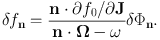
where [..] denotes the Poisson bracket. Writing f(J, θ, t) = f₀(J) + f₁(J, θ, t) and H(J, θ, t) = H₀(J) + H₁(J, θ, t), we have to first order

(1.76)

We note that ∂ H₀ / ∂ θ = Ω₀ and Fourier expand H₁ and f₁

(1.77)

where by virtue of the time-translation invariance of equation (1.76) we have assumed that all perturbed quantities have the same frequency, ω. Using these expansions in equation (1.76) we equate coefficients of e^{i(n · θ − ω t)} on each side to obtain

(1.78)

The frequencies ω of the system's normal modes are determined by the requirement that Φ₁ is related by Poisson's equation to the density fluctuation implied by f₁. This requirement reads

(1.79)

This equation is homogeneous in δΦ_n so we expect it to have non-trivial solutions only for particular values of ω, the frequencies of normal modes. Finding the normal-mode frequencies is hard because the equation involves in an essential way two systems of phase-space coordinates: (x, p) and (θ, J).

Although equation (1.79) can be tackled (see for example Kalnajs, 1977, Read & Evans, 1998), we will pursue a simpler course. We restrict ourselves to razor-thin discs, which have a four-dimensional phase space, and use the tight-winding approximation. We assume that the disturbance is a tightly wound spiral wave, so

(1.80)

with kR ≫ 1 for trailing waves and kR ≪ −1 for leading waves. It is straightforward to show from Poisson's equation that the corresponding surface density is

(1.81)

We adopt the epicycle approximation (§ 1.1.3), in which the real-space coordinates are related to angle-action coordinates by

(1.82)

where

(1.83)

Then the Fourier decomposition of Φ₁ is

(1.84)

We now combine the two exponentials of circular functions into a single exponential of a single cosine and use equation (8.511.4) of Gradshteyn & Ryzhik (1965) to express this as a sum over Bessel functions _l. Specifically

(1.85)

where α is the pitch angle and is the total wavenumber of the spirals:

(1.86)

Using equation (1.85) to rewrite equation (1.84) we obtain

(1.87)

Equation (1.87) tells us what δΦ_n(J) is for n = (l, m, 0):

(1.88)

Using this in equation (1.78) we obtain the change in the DF caused by Φ₁:

(1.89)

The change in the surface density is Σ₁ = ∫ d² p f₁. Since our expression for f₁ uses angle-action coordinates rather than (x, p) coordinates, we use a trick based on the fact that d² x d²p = d² θ d²J because both systems are canonical:

(1.90)

Using equation (1.82) for φ′ and R′, and equation (1.89) for δ f_n, this becomes

(1.91)

The two Dirac delta-functions enable us to carry out the integrals over θ_φ and J_φ. This done every occurrence of R_g(J_φ) (including those in the definitions of κ, a, etc.) should, strictly, be replaced by R − a cosθ_r. However, the tight-winding approximation allows us to neglect the small difference between R_g and R except when it occurs in the argument of an exponential multiplied by the large number k. With the aid of this approximation we obtain

(1.92)

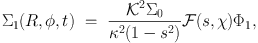
It is simple to show that dJ_φ / dR_g ≡ dL_z / dR_g = R_g κ/γ. For f₀ we adopt

(1.93)

which with the epicycle approximation (eq. 1.82) yields the Schwarzschild velocity distribution with radial dispersion σ (e.g. §4.4.3 Binney & Tremaine, 2008, Binney, 2010). Finally, we use equation (1.85) to express the exponential of sinusoids in the last line of equation (92) as a sum over Bessel functions. Then we can evaluate the integral over θ_r to obtain

(1.94)

where equation (6.615) of Gradshteyn & Ryzhik (1965) has been used to evaluate the integral over J_r, I_l is a modified Bessel function, and

(1.95)

Two more definitions and the identity I_l(z) = I_−l(z) enable us to write equation (1.94) in the neater form

(1.96)

where

(1.97)

The final step is to require that the value of Σ₁ from equation (1.96) agrees with that given by equation (1.81). Eliminating Σ₁ between these equations and approximating by |k| (see eq. 1.86), we obtain the Lin-Shu-Kalnajs dispersion relation for tightly wound spiral waves:

(1.98)

For an m-armed spiral with pattern speed Ω_p, ω = m Ω_p so

(1.99)

which rises from −1 at the ILR through zero at the CR to 1 at the OLR. Hence from equation (1.98) k vanishes at the Lindblad resonances. One finds that behaves roughly as k(1 − b k) with b > 0, so the left side of the dispersion relation peaks for some k, and Toomre (1964) showed that if the disc is stable to axisymmetric disturbances this peak value is smaller than unity, so solutions for k cannot be found for a range of small values of s². Thus waves are forbidden in a zone around the CR as well as inside the ILR and outside the CR. In the permitted zones two values of k can be found for given s, the values approaching one another as s approaches the forbidden zone around the CR. Thus there are two branches to the dispersion relation, and the branches merge at the edge of the CR zone.

When Toomre (1969) determined the group velocity of waves from the dispersion relation, he found that short-leading waves propagate outwards from the ILR. At the edge of the forbidden region around the CR these waves transfer to the long-leading branch and propagate back towards the ILR. As the waves approach the ILR, k decreases and the validity of the tight-winding approximation becomes questionable. If it remains valid, the waves reflect off the ILR into long-trailing waves, which propagate out towards the CR. At the edge of the CR's forbidden region the waves morph into short-trailing waves, which propagate back towards the ILR. As they approach the ILR k is predicted to grow without limit. In reality the wave is absorbed as it approaches the ILR and its energy dissipates as heat. Thus the tight-winding approximation predicts that short-leading waves gradually wind up into short-trailing waves, which heat the disc in the vicinity of the ILR. The unwinding of leading waves and winding-up of trailing waves is similar to what differential rotation would do to material arms.

Similarly, the dispersion relation implies that short leading waves will propagate inwards from the OLR to the outer edge of the forbidden region around the CR, where they will transfer to the long branch of the dispersion relation and move back out as long leading waves. If the tight-winding approximation remains valid as they approach the OLR, they will morph into long trailing waves that propagate back inwards towards the CR and then return as short trailing waves that eventually thermalise at the OLR.

As waves transfer from leading to trailing form near a Lindblad resonance, the waves morph from elongated ridges of overdensity to compact blobs of over-density. If Toomre's

(1.100)

is small enough, self-gravity imparts a sharp inward impulse to these blobs, so their density begins to rise. Simultaneously, differential rotation is shearing them into trailing waves, which propagate away from the resonance. Consequently, the waves that reach the forbidden zone around the CR have larger amplitude than the waves that left this zone earlier. We say the waves have been swing amplified. Our formulae do not predict this behaviour because they rely on the tight-winding approximation, which is invalid at the crucial moment.

The gain of the swing amplifier is a sensitive function of Q and the parameter

(1.101)

where k_crit is defined by equation (1.98). The smaller X is, the more invalid the tight-winding approximation, and the smaller Q is, the cooler the disc. The disc is stable to axisymmetric disturbances only if Q > 1. ⁴ Swing amplification by a factor >10 is possible for Q ≲ 1.5 and X ≲ 3.

Since a key phase in the life-cycle of waves that we just described, the waves are unlikely to satisfy the tight-winding approximation, it is natural to ask about solutions of the fundamental equation for normal modes, eq. (1.79). Toomre (1981) reported results obtained in this way by his student T. Zang. These showed that when the growth rate of a mode is not large, the mode looks like an interference pattern between leading and trailing waves that differ only in their amplitude, the trailing wave having the larger amplitude. The larger the mode's growth rate is, the more the trailing waves dominates. This finding is consistent with swing amplification taking place as disturbances morph from leading to trailing. Another finding was that the modes are essentially confined to the region between the ILR and the CR. Read & Evans (1998) solved for the normal modes of discs with power-law gravitatinal potentials. They also found that the amplitudes of modes are largest between the ILR and the CR. Their models had “cut-out” discs, that is discs whose surface density tapered to negligible values at both very small and very large radii. The growth rate of a mode depended strongly on whether the ILR lay inside the inner cut-out, that is in a region of low density. In this case inward propagating short-trailing waves can reflect off the inner edge of the disc into leading waves, thus closing a feedback loop, rather than being absorbed at the ILR. Thus solutions to our mode equation (1.79) lend support to the qualitative understanding of spiral structure provided by the dispersion relation for tightly-wound waves.

The bottom line is that stellar discs are responsive dynamical systems because they support waves that can be amplified by self gravity as they move through the disc. The degree of amplification, and therefore the disc's responsiveness, increases sharply as the velocity dispersion falls towards the critical value at which Q = 1 and the disc becomes unstable to radial fragmentation. Much of the energy carried by the waves is thermalised in the vicinity of a Lindblad resonance. Thus the waves heat the disc and render it less responsive.

1.4.3. Spiral structure and normal modes

Lin & Shu (1966) hypothesised that spiral structure is a manifestation of a mildly unstable normal model of the stellar disc: they envisaged the amplitude of this mode stabilising at a finite value as a result of energy dissipation in interstellar gas. They developed the theory of density waves in the expectation that the normal modes of discs could be understood in terms of waves trapped between barriers in the same way that we picture the modes of a laser as standing waves trapped between the laser's end mirrors. It's now clear that the very influential Lin–Shu paradigm is based on a misunderstanding of disc dynamics. Waves in a stellar disc are heavily damped already at the level of stellar dynamics because they heat the disc at the Lindblad resonances.

From a certain perspective the failure of the Lin–Shu hypothesis is perplexing: stellar dynamics is governed by the coupled Poisson and collisionless Boltzmann equations. These equations are time-translation invariant, so on group-theoretic grounds their linearised forms must have a complete set of solutions with time dependence e^{ν t}, with ν possibly complex. Unless the system is completely stable, the evolution from any initial condition will be dominated by the most rapidly growing normal mode. Hence the observations must reflect such modes.

The problem with this argument is that it assumes that any initial configuration can be represented by a superposition of normal modes. In other words, the normal modes are assumed to be complete. The solutions to our normal-mode equation (1.79) are not complete because in deriving it we have used defective logic: equation (1.78) is obtained by dividing both sides of

(1.102)

by n · Ω − ω. This operation is legitimate only if n · Ω − ω ≠ 0. If we want our normal modes to be complete, we have to include the case n · Ω − ω = 0 and replace equation (1.78) by

(1.103)

In the simpler but closely analogous case of an electrostatic plasma, van Kampen (1955) was able to show that by considering such singular DFs Poisson's equation can be satisfied for any real value of ω. In this way we obtain a much richer set of solutions than can be obtained from equation (1.78). All these van Kampen modes are stable, and they prove to be complete, whereas the solutions we would obtain from equation (1.78) are incomplete and as such do not form a basis for a discussion of stability.

1.4.4. Driving spiral structure

By counting faint stars in the outer reaches of both our Galaxy and the Andromeda nebula, M31, it has been shown that the outer parts of galaxies are a mass of stellar streams and full of faint satellite galaxies (McConnachie et al., 2009, Belokurov et al., 2006, Bell et al., 2008). From studies of the internal dynamics of satellite galaxies, we know that these systems are heavily dominated by dark matter, so we must anticipate that the dark-matter distribution that surrounds a galaxy like the Milky Way is lumpy. When a lump of dark matter sweeps through pericentre, its tidal field will launch a wave into the host galaxy's disc, which we know to be a responsive system. The classic example of this process in M51, which has a satellite galaxy, NGC 5195, near the end of one of its exceptionally strong spiral arms. Few galaxies have such a luminous satellite so near to them, so grand-design spirals like that of M51 are not prevalent. Most galaxies will be responding simultaneously to more than one much weaker stimulus, with the result that their spirals are both weaker and rather chaotic.

A majority of spiral galaxies have bars at their centres. The figures of bars are known to rotate quite rapidly in that the CR of the bar's pattern lies at a radius that is ∼ 1.2 times the bar's length. The rotating gravitational field of the bar must perturb the disc, and from the discussion of § 1.4.2 we would expect the surrounding disc to show spiral structure at the pattern speed of the bar that extends from near the end of the bar to the OLR. However, both N-body simulations and observations show that the disc's principal response is at a lower pattern speed than that of the bar (Sparke & Sellwood, 1988), so bar excites spiral structure that lies inside its CR. This finding is consistent with the tendency of the solutions to the normal-mode equation (1.79) to have significant amplitudes only inside CR. Crucially it implies that the response to the bar rotates more slowly than the bar, so the relative phases of the features is constantly changing.

⁴ We can show this from equation (1.98) by setting m = 0. Back.