4. OBSERVATIONAL DIAGNOSIS OF THE COOL ISM IN DISTANT GALAXIES

4.1. Molecular gas excitation

As noted in Sec. 2.6 the excitation of molecular gas in high–redshift galaxies provides important information regarding the average physical properties of the gas, in particular its temperature and density. This is illustrated in Fig. 3 where the expected CO excitation is shown as a function of density and temperature. One important caveat is that typically only galaxy–integrated line fluxes can be measured at high redshift. These measurements are then fed into LVG (Sec. 2.6.1) or PDR/XDR (Sec. 2.6.2) models that assume that the line emission is emerging from the same cloud/volume (i.e. that they share the same physical conditions). The validity of this assumption is questionable, as it is known that the different rotational transitions have different critical densities: the higher–J transitions need much higher densities than the low–J ones to be excited. This situation complicates further if unresolved measurements of high–density tracers (e.g. HCN, HCO⁺) are added to the ‘single component' models. Another caveat is that the molecular gas excitation measurements in high redshift galaxies are typically restricted to the mid–J levels of CO emission.

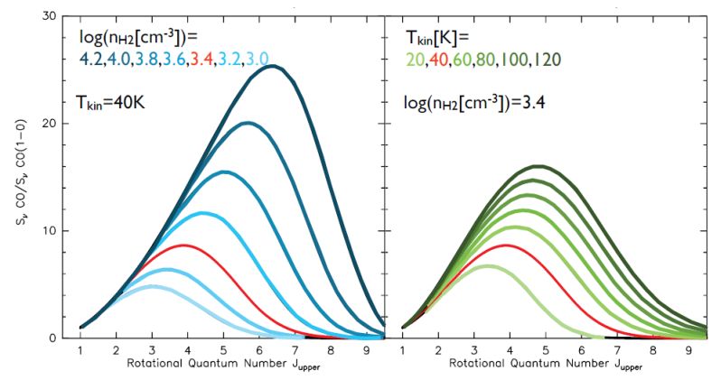Figure 3. This figure illustrates how the measured CO emission ladder changes as a function of temperature and density (adopted from Weiß et al. (2007). The left panel shows the effect of changing density at fixed temperature (Tkin = 40 K. The right panel shows the effect of varying kinetic temperatures for a fixed density (log(n(H2)) = 3.4). Both panels have been normalized to the CO(1–0) transition. High CO excitation is achieved through a combination of high kinetic temperature and high density. Given the typically sparsely sampled CO excitation and large error bars in high redshift observations, this degeneracy can not be easily broken observationally. Additional information, such as independent estimates of the kinetic temperature through [C I] or dust measurements can help to break this degeneracy. Note that increased temperatures lead to a broader CO emission ladder, as more and more high–J levels are populated following the Boltzmann distribution.

With these caveats in mind there are a number of important results emerging from high–redshift CO excitations analyses. The main result is that the different source populations at high redshift show distinctly different excitation (see compilation of all high–redshift CO excitation in Fig. 4). The CO excitation of quasar host galaxies can in essentially all cases be modeled by a simple model with one temperature and density out to the highest–J CO transition with a typical gas density of log(n(H₂)[cm⁻³]) = 3.6 – 4.3, and temperatures of T_kin = 40−60 K. A prominent example is the highly excited quasar host APM 08279+5255 (Weiß et al. 2007a). Measurements of the CO ground transition in a number of quasar host galaxies (Riechers et al. 2011a) have shown that the measured CO(1–0) flux is what was expected based on a single–component extrapolation from higher–J CO transitions, i.e. there is no excess of CO(1–0) emission in these sources (Riechers et al. 2006a, 2011a). One interpretation of this finding is that the molecular gas emission comes from a very compact region in the centre of the quasar host, which is confirmed by the few (barely) resolved measurements of quasar hosts (Sec. 4.6). It should be noted though that there is recent evidence that an additional high–excitation component, likely related to the AGN itself, is needed to explain the elevated high–J line fluxes in some sources, e.g. PSS 2322+1944 (Weiß et al., in prep.) and J 1148+5251 (Riechers et al., in prep.).

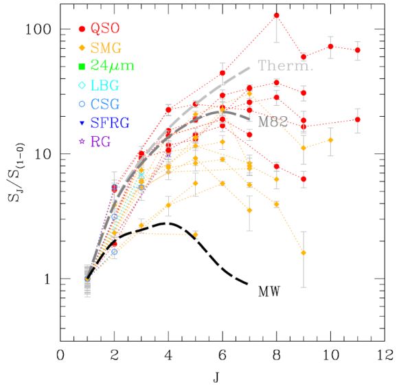Figure 4. CO emission ladder of all sources where the CO(1–0) line has been measured. The CO line flux is shown as a function of rotational quantum number and the colors indicate the different source types. Measurements for individual sources are connected by a dashed line. The line fluxes have been normalized to the CO(1–0) line. The QSOs are the most excited systems found, with an average peak of the CO ladder at around J ∼ 6. This is consistent with the high star formation rate and compact emission regions in their host galaxies. The SMGs are slightly less excited on average, and their CO emission ladder peak around J ∼ 5. The dashed thick lines indicate template CO emission ladders for the Milky Way (black) and M 82 (grey). The dashed dark grey line shows constant brightness temperature on the Rayleigh–Jeans scale, i.e. S ∼ ν2 (note that this approximation is not valid for high J).

The submillimeter galaxies, on the other hand, show (i) less excited molecular gas, and (ii) excess emission in the CO(1–0) ground transition. This is again illustrated in Fig. 4, where the orange symbols of the SMGs are on average at lower fluxes compared to the quasars (red symbols). On average, the typical density of SMGs is log(n(H₂)[cm⁻³]) = 2.7-3.5, and temperatures are in the range of T_kin = 30 − 50 K. Observations in the CO(1–0) line of a few SMGs have furthermore demonstrated that an additional cold component is needed to explain the observed excitation (Ivison et al. 2011, Riechers et al. 2011b). This implies that the total gas mass of the SMGs is underestimated if mid–J CO transitions are used to calculate masses assuming constant brightness temperature (see Sec. 4.2). A few SMGs have been resolved spatially and show more extended emission in the ground transition than in higher transitions (Ivison et al. 2011; although cf. Hodge et al. 2012).

Up to the mid–J measurements available for high redshift sources the CO excitation of the SMGs and QSOs roughly follow those of the centres of nearby starburst galaxies (e.g., M 82: Mao et al. 2000; Ward et al. 2003, see dashed line in Fig. 4; NGC 253: Bradford et al. 2003; Bayet et al. 2004, and Henize 2-10: Bayet et al. 2004). It should be noted that the excitation in Galactic molecular cloud cores can be equally high (e.g. Habart et al. 2010, Leurini et al. 2012; van Kempen et al. 2010, Manoj et al. 2012). However, in Galactic clouds such very high excitation is only seen in pc scales cloud cores, while in nearby starburst nuclei high excitation is seen on scales of order 100 pc scales, and for high–redshift galaxies the scale can extend to a few kpc.

As stated in Sec. 3, the seperation between SMGs and QSO host galaxies is largely due to historical selection effects and there are sources that fullfill both definitions. The different excitation conditions in the two groups however argue that broadly speaking gas–rich quasars and SMGs represent different stages of galaxy evolution, with the quasars being more compact and harboring more highly excited gas than the SMGs. In a simplistic picture, the quasars could be the result of a merger, in which the molecular gas concentrates in the centre of the potential well, while the SMGs would then constitute merging systems that have not fully coalesced. The latter is supported by the fact that high–resolution observations of many SMGs show multiple emission components (e.g. Engel et al. 2010, Tacconi et al. 2010). SMGs and quasars also show similar clustering properties (Hickox et al. 2012).

To date, only a few excitation measurements exist for the CSGs (Dannerbauer et al. 2009; Aravena et al. 2010), and only up to CO 3-2. In the case of BzK-21000 Dannerbauer et al. (2009) showed that the J = 3 emission must be significantly subthermally excited, resembling more that of the Milky Way than the higher–excitation systems discussed above. These CSGs have lower star formation rates than found in the quasars and SMGs, and have large ( ∼ 10 kpc) sizes – the combination of these apparently leads to a less extreme gas excitation than found in the hyper-starburst galaxies at high redshift. Observations of higher order CO transitions are required in these systems.

Bothwell et al. (2012) suggest that there is a correlation between CO luminosity and line width in high redshift starbursts, likely relating to baryon-dominated gas dynamics within the regions probed. In Fig. 5, we plot the CO line widths (FWHM) vs. CO luminosity for a broader range of CO detected distant galaxy types. Considering only the hyperstarbursts (SMGs and quasar hosts), both occupy similar parameters space in this diagram, and there is no significant correlation between CO luminosity and linewidth. However, the CSG clearly segregate to smaller line widths relative to SMGs, by about a factor ∼ two, and, while the scatter is large, the median CO luminosity for CSGs is smaller by a similar factor.

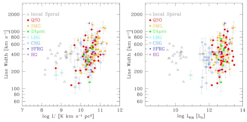Figure 5. The CO line width (FWHM) versus CO line luminosity (left) and versus the FIR luminosity (right panel). Note that the CSG show systematically lower line widths for a given CO line luminosity than the hyper–starburst quasar hosts and SMGs (we have corrected the vrot, max values given in Tacconi et al. (2010) to give accurate FWHM values). The grey datapoints show local spiral galaxies (with stellar masses > 1010 M⊙ from the HERACLES/THINGS surveys (Leroy et al. 2008, Walter et al. 2008). The local FWHM values are corrected for inclination, the high–z values are not (in the absence of unknown inclinations).

4.2. CO luminosity to total molecular gas mass conversion

Until a few years ago, the standard practice for high redshift galaxies was to use the starburst conversion factor to derive gas masses. This practice was justified in part on the extreme luminosities, high inferred gas densities based on CO excitation, and in some cases on the direct observation of compact star forming regions (scales ∼ 2−4 kpc; Tacconi et al. 2008, Momjian et al. 2007, Ivison et al. 2010a, 2012, Carilli et al. 2002, Walter et al. 2009). Also, in some cases it appeared that, like nearby nuclear starbursts, the gas mass exceeded the dynamical mass when using a Milky Way conversion factor (Solomon et al. 1997, Tacconi et al. 2008, Carilli et al. 2011, Walter et al. 2004, Riechers et al. 2008, 2009).

As other populations of galaxies are now being detected in CO emission at high redshift, such as color–selected star forming galaxies (Sec. 3.5), the question of the conversion factor has become paramount. The last few years have seen a few attempts at the first direct measurements of the CO luminosity to gas mass conversion factor.

A minimum α can be derived assuming optically thin emission, and adopting a Boltzmann distribution for the population of states. In this case, the CO(1–0) luminosity, L_CO(1−0), simply counts the number of molecules in the J = 1 state via: N_J=1 = L_CO(1−0) / (A × hν), where A is the Einstein A coefficient (6 × 10⁻⁸ s⁻¹), and ν = 115 GHz. The total number of CO molecules is then determined by the partition function, ie. the relative fraction in the J = 1 state, which we designate f. For example at T = 10, 20, and 40 K, f = 0.47, 0.31, and 0.19, respectively. One can then convert to total number of H₂ molecules assuming a CO/H₂ abundance ratio, which for Galactic GMCs is 10⁻⁴. Multiplying by the mass of an H₂ molecule, and including a factor 1.36 for the Helium abundance, leads to the total gas mass. Converting to the relevant units, leads to: α = (0.09 / f) M_⊙ [K km s⁻¹ pc²]⁻¹, at z = 0. ¹

Tacconi et al. (2008) use spatially resolved spectral imaging to derive either virial or rotational masses for a sample of SMGs and color selected galaxies. Galaxy sizes are estimated from the CO imaging and/or optical or near–IR imaging (see also Neri et al. 2003; Thomson et al. 2012). Tacconi et al. compare the dynamical masses with the sum of the gas mass (modulo α) and stellar mass (derived from near–IR photometry), including a small correction (10% to 20%) for dark matter. They conclude that for the SMGs, the value of α is most likely close to the starburst value (α ∼ 1), while for the CSG a value α ∼ 4.8 is favored.

Daddi et al. (2010) have performed a similar analysis on CSGs, based on (marginally) spatially resolved imaging with the PdBI of CO 2–1 emission of a sample of three z ∼ 1.5 sBzK galaxies. Their dynamical analysis is guided by numerical simulations of clumpy, turbulent disks, to allow for significant non–circular motions (Bournaud et al. 2009). They find that the measurements are consistent with α_CO = 3.6 ± 0.8 M_⊙ / (K km s⁻¹ pc²).

The best rotational dynamical analysis of an SMG to date is the JVLA observation of GN 20 at z = 4.0 (Fig. 7) by Hodge et al. (2012; see Sec. 4.6). They show that the CO(2–1) emission is well characterized by a rotating disk of 7 kpc radius with a large rotation velocity of 575 ± 100 km s⁻¹ and internal velocity dispersion of 100 km s⁻¹. They derive a dynamical mass of 5.4 ± 2.4 × 10¹¹ M_⊙. Subtracting the stellar mass, including a 15% dark matter contribution leads to α ∼ 1 M_⊙ / (K km s⁻¹ pc²).

The main uncertainties in the dynamical analysis are the current crude estimates of the dynamical masses based on marginally resolved imaging data, and the standard pit–falls in estimating the stellar masses based on SED fitting, in particular for starburst–type systems (Ivison et al. 2011).

Magdis et al. (2011) use a metallicity–dependent dust–to–gas ratio approach to estimate α_CO. They analyze two galaxies in the GOODS–N deep field with excellent rest–frame IR SEDs, one SMG (GN 20), and one CSG (BzK-21000). From these, and using the Draine & Li (2007) dust models, they derive a dust mass for each source. Metallicities are derived from the stellar mass – metallicity relation for the CSG (Erb et al. 2006), and a starburst model for GN 20. They then use the Solomon et al. (1997) metallicity dependent dust to gas relation to obtain an estimate of the gas masses of 9 × 10¹⁰ M_⊙ for the CSG and 1.5 × 10¹¹ M_⊙ for the SMG. Comparing these masses to the CO(1–0) luminosities leads to α ≤ 1.0 for the SMG, while for the CSSGF they find α ∼ 4, consistent with earlier estimates. These results have been generalized in the more comprehensive study by Magdis et al. (2012b).

Ivison et al. (2011) take two different approaches to derive molecular gas masses, and hence infer α in SMGs. First, they propose a model in which some fraction of the CO emission occurs at the ‘Eddington limit' in dense star forming regions (a ‘maximal starburst'), ie. a self–gravitating disk supported by starburst–driven radiation pressure on the dust grains (Thompson et al. 2005; Thompson 2009; Krumholz & Thompson 2012). Thompson (2009) derive a maximum star formation efficiency in this case of: SFE_max ≡ L_IR / M_gas < 500 L_⊙ M_⊙⁻¹, and an areal star formation rate density of 1000 M_⊙ yr⁻¹ kpc⁻². This maximum surface density is seen to hold on scales from star forming cloud cores in GMCs ( ∼ 1pc) to the nuclear starburst regions of low–z ULIRGs.

Ivison et al. then make a correction to the total gas for the fraction of cold, quiescent gas not involved in active star formation based on the CO excitation. Under these assumptions, the molecular gas mass can be estimated from the IR luminosity. For 4 of their 5 SMGs, the values are between α = 0.4 and 0.7, while for the last source the value is 3.7. This latter source also has by far the lowest CO excitation.

Second, Ivison et al. (2011) use radiative transfer modeling to derive physical conditions within the clouds, and infer gas masses in a manner analogous to the low redshift ULIRG analysis of Downes & Solomon (1998). Unfortunately, LVG models have a fundamental degeneracy between density, temperature, and non–virial gas kinematics, when using just CO excitation (Sec. 2.6.1). They find the CO SEDs are consistent with either α ∼ 4.5 in cold, dense gas with large non–virial motions, or α ∼ 1 in warm, more diffuse gas closer to virial dynamics.

Genzel et al. (2012) consider the effect of metallicity on the conversion factor α in a sample of CSG at z ∼ 1 to 2. They have obtained estimates for the metallicities from optical [N II]/Hα measurements. They find that galaxies with similar sizes, SFRs, and dynamical masses, but different metallicities (and stellar masses; Erb et al.), show very different star formation efficiencies, with the CO to FIR luminosity ratio decreasing dramatically with decreasing metallicity, at fixed FIR luminosity. If α is the same in each system, then this would imply a much shorter gas consumption timescale (gas mass/SFR) in low metallicity galaxies vs. high metallicity galaxies.

Alternatively, Genzel et al. (2012) propose adopting a standard star formation efficiency relating gas mass to star formation rate (Sec. 4.5). In this case, the decrease in CO luminosity is not due to a lower gas mass but an increase in α at low metallicity. Such a trend is expected and observed at low metallicity in nearby galaxies (Sec. 2.5), since dust shielding becomes less efficient, and CO in molecular cloud envelopes are photo–dissociated much more deeply into the cloud (Leroy et al. 2011; Bolatto et al. 2013, Schruba et al. 2012). Genzel et al. 2012; Stacey et al. 1991) derive the empirical relationship: log(α_CO) = 12 − 1.3 × [12 + log(O/H)]. The implication is that stars can form in CO–poor molecular gas, and that the expected CO luminosities of low metallicity galaxies at high redshift are lower than previously predicted based on standard α values (Glover & Clark 2012; Papadopoulos & Pelupessy 2010).

Magnelli et al. (2012) perform a similar analysis of the conversion factor based on dust-to-gas ratios, for a mixed sample of SMGs and CSG at z = 1 to 4. They adopt a similar dust mass calculation based on the FIR luminosity, and a metallicity-dependent dust-to-gas ratio as in Genzel et al. (2012). Their results are consistent with a low value of α for starbursts, and a factor five higher value for CSG. They also find a trend of decreasing α with increasing dust temperature, and while the trend may be continuous, they recommend that for a dust temperatures < 30K, a Milky Way conversion factor is appropriate, while for higher dust temperatures the starburst value should be used, at least for solar metallicity systems.

Many conclusions in astronomy are not based on a single, absolutely compelling direct measurement, but on a series of measurements, modeling, and consistency arguments from which the weight of evidence leads to a ‘concordance model'. This approach applies to the the CO–to–gas mass conversion factor in distant galaxies. The current measurements of α_CO are principally based on dynamical imaging and modeling, dust–to–gas measurements, radiative transfer modeling, and most recently, on star formation efficiencies. These measurements suggest a nuclear starburst value ∼ 0.8 M_⊙ / (K km s⁻¹ pc²)⁻¹ for SMGs and quasar hosts, and a Milky Way GMC value of α_CO ∼ 4 M_⊙ / (K km s⁻¹ pc²)⁻¹ in CSG, with a likely further increase in low metallicity galaxies. These values are consistent with the generally extended, clumpy disk–like CO distribution, lower CO excitation, and Milky Way CO/FIR (FIR derived from SFR) ratios in CSG, compared to the often (although not exclusively) more compact, merger–like morphologies, higher excitation, and starburst CO/FIR ratios in SMGs and quasars.

4.3. Atomic Fine Structure lines

4.3.1. Atomic Carbon: [C I] In a recent study, Walter et al. (2011) summarize the [C I] observations of 13 high–redshift galaxies (this compilation included work by Barvainis et al. 1997, Weiß et al. 2003, 2005a, Pety et al. 2004, Wagg et al. 2006, Ao et al. 2005, Riechers et al. 2009a, Casey et al. 2009, Lestrade et al. 2010, Danielson et al. 2011). These systems studied in [C I] are amongst the brightest emitters both in the submillimeter regime and in CO line emission, and many of them are lensed. The main finding was that the [C I] properties of high–redshift systems do not differ significantly to what is found in low–redshift systems, including the Milky Way. In addition, there are no major differences in [C I] properties between the QSO– and SMG–selected samples. The L′_CI(1−0) / L′_CO ratios (0.29 ± 0.12) are similar to low–z galaxies (e.g., 0.2 ± 0.2, Gerin & Phillips 2000).

As argued in Sec. 2.8, measurements of both [C I] lines can constrain gas excitation temperatures of the molecular gas, independent of radiative transfer modeling. For the available sample, a carbon excitation temperature of 29.1 ± 6.3 K was derived (Walter et al. 2009). This temperature is lower than what is typically found in starforming regions in the local universe despite the fact that the sample galaxies have star formation rate surface densities on kpc scales of 100's of M_⊙ yr⁻¹ kpc⁻². However, the temperatures are roughly consistent with published dust temperatures of high–redshift starforming galaxies (Beelen et al. 2006, Kovács et al., 2006, 2010, Harris et al. 2012). Low carbon excitation as well as low dust temperatures could indicate that the measurements include a significant amount of gas/dust unaffected by star formation.

The [C I] abundances in the current high–z galaxy sample of (X[[C I]] / X[H₂] = (8.4 ± 3.5) × 10⁻⁵) are comparable, within the uncertainties, to what is found in local starforming environments (Walter et al. 2009). The [C I] lines are a negligible coolant (average L_CI / L_FIR = (7.7 ± 4.6) × 10⁻⁶). There is tentative evidence that this ratio may be elevated in the SMGs by a factor of a few compared to the QSOs (Walter et al. 2009).

4.3.2. Ionized Carbon: [C II] The [C II] 158µm line is rapidly becoming a work–horse line for the study of the cool atomic gas in distant galaxies. The number of [C II] detections at high redshift has increased substantially in the last few years using the CSO, PdBI, APEX and the SMA (Maiolino et al. 2009; Stacey et al. 2010; Iono et al. 2006b, Hailey–Dunsheath et al. 2010, Wagg et al. 2010; Walter et al. 2012; Cox et al. 2011; De Breuck et al. 2011; Gallerani et al. 2012), as well as a few detections in strongly lensed galaxies with Herschel (Ivison et al. 2010b, Valtchanov et al. 2011). To date, there have been about two dozen [C II] detections from galaxies at z > 1, including a number at z > 6 (see Sec. 5.2). ALMA during early science has already demonstrated the ability to detect [CII] emission from relatively normal star forming galaxies at high redshift (LBGs, LAEs) in [C II] emission (Wagg et al. 2012; Carilli et al. 2012; Riechers et al. 2013).

Fig. 6 shows a broad scatter in the [C II] / FIR ratio at z > 1. Note that the high–z galaxy sample all have FIR luminosities ≥ 10¹² L_⊙. However, there is a trend for luminous AGN to have the lowest ratios, and star–formation dominated galaxies (eg. SMGs) to have ratios closer to that of the Milky Way (e.g., Stacey et al. 2010).

Figure 6. The ratio LCII / LFIR as a function of LFIR (data from Table 3). The dashed horizontal line indicates a value of 3 × 10−3 ∼ Milky Way value. The LFIR measurements are corrected for lensing (where known).

Stacey et al. (2010) use the CO, FIR, and [C II] emission to argue that the [C II] emission is dominated by PDRs in the star forming galaxies. From these observations, they derive the physical conditions in the PDRs in high redshift galaxies, finding gas densities of order a few × 10⁴ cm⁻³, and the strength of the FUV radiation field: G ∼ 10³ × 1.6 × 10⁻³ erg cm⁻² s⁻¹, where 1.6 × 10⁻³ erg cm⁻² s⁻¹ is the local Galactic interstellar radiation field (ISRF, ‘Habing field'). They find a further factor 10 higher G for the AGN dominated systems. Their modeling also implies that the scale of the PDRs is ≥ few kpc, much larger than for GMCs or nuclear starburst galaxies at low redshift. The fraction of molecular gas mass associated with PDRs is between 20% and 100% in their sample.

Swinbank et al. (2012) detect likely [CII] 158µm emission in two SMGs using ALMA, from which they derive redshifts of z ∼ 4.4 and 4.2. They suggest that the bright-end of the [CII] luminosity function increases dramatically with redshift, with close to a thousand-fold increase in the number density of galaxies with L[[CII] > 10⁹ L_⊙ from z = 0 to 4. We discuss [CII] detections in a number of z > 6 galaxies in Sec. 5.2.

4.3.3. Other fine structure lines There have been only a few detections of fine structure lines other than [C II] at high redshift to date, mostly in strongly lensed systems using principally the PdBI and Herschel. We summarize some of the physical diagnostics that have been achieved with such observations.

In their Herschel study of SMGs at z ∼ 1.4, Coppin et al. (2012) find that the [O I] 63 µm / FIR ratio is comparable to spiral galaxies nearby, and much higher than what is seen in low–z nuclear starbursts. Similar results were found by Ferkinhoff et al. (2010) and Sturm et al. (2010) in their [O I] 63µm, [O III] 52µm, and [C II] 158µm study of a strongly lensed ULIRG at z = 1.3 (see also Hailey–Dunsheath et al. 2010). The interesting conclusion is that, although these systems are intrinsically ULIRG or HyLIRGs, they do not show a deficit in the major PDR cooling lines as seen in nearby ULIRGs. A similar conclusion has been reached based on [C II] and [N II] observations of lensed SMGs (Nagao et al. 2012; De Breuck et al. 2011). In particular, the compilation of Decarli et al. (2012) shows a mean value for [N II] 122µm / FIR ∼ 3 × 10⁻⁴, close to that seen in low z disk galaxies, although admittedly the scatter is large.

Conversely, Valtchanov et al. (2011) and Ferkinhoff et al. (2010; 2011) perform PDR analyses of lensed SMGs at z ∼ 3, using FIR, CO, [O III] [N II] and/or [C II] measurements. They find mean densities of order 2000 cm⁻³, FUV radiation field of G = 200, and sizes for the emitting region ∼ 0.6 kpc. The relatively strong [O III] implies that the radiation field must be very hot (35,000K), either dominated by O9.5 stars or an AGN NLR–like radiation field.

The [C II] 158µm line is realizing its potential in the study of the cooler atomic gas in distant galaxies. This strong line will be a workhorse–line for redshift determinations in the first galaxies, and in the study of galaxy dynamics at the highest redshifts. However, the interpretation of [C II] emission is not straighforward, since [C II] traces both the neutral as well as the ionized medium, and it appears to be suppressed in high–density regions. Likewise, multi–fine structure line diagnostics at high redshift have tremendous potential to probe the physical conditions in the ISM in high z galaxies, but studies are in their infancy. The current observations reflect the heterogeneous nature of SMGs, with many showing spiral galaxy–like FSL properties, and a few showing evidence for an AGN–like component.

4.4. Dense gas tracers and other molecules at high redshift

Emission from high dipole molecules, such as HCN and HCO⁺, comes only from highest density regions in molecular clouds (n_cr > 10⁴ cm⁻³), corresponding to regions directly associated with active star formation. These lines are typically an order of magnitude weaker than the integrated CO emission from star forming galaxies, although the higher dense gas fraction in nuclear starbursts can lead to line strengths up to 25% of CO (Riechers et al. 2011c). To date, there remain just a handful of detections at high redshift, mostly from strongly lensed hyper–starbursts (Riechers et al. 2006b, 2010c; 2011c; García-Burillo et al. 2006, Danielson et al. 2011). The two strongly lensed hyper-starburst/AGN, APM 0827+5255 at z = 3.91 and the Cloverleaf quasar (H1413+117; Barvainis et al. 1994) at z = 2.56 play an analogous role to the Galactic molecular cloud SgrB2, as high–z ‘molecule factories'. These are the only sources with multiple transitions detected from molecules and isotopes other than ¹²CO, including HCN, HNC, HCO⁺, H₂O, CN, ¹³CO. We briefly review the recent results on these sources.

For APM 0827+5255, strong emission from very high order transitions is seen (Weiß et al. 2007a; Riechers et al. 2010c). Formally, the critical densities for excitation for the higher order HCN and HCO⁺ transitions are > 10⁸ cm⁻³. The excitation suggests emission from a region with a radius ∼ 200 pc around the AGN, where IR pumping (Sec. 4.4) plays a dominant role in molecular excitation. The J = 6 isomer ratio of HNC/HCN = 0.5 is consistent with the IR pumping model (Riechers et al. 2010c).

For the Cloverleaf quasar, low and high order emission from HCN and HCO⁺, and CN have been detected (Solomon et al. 2003; Riechers 2006b, 2007a, 2011c; Barvainis et al. 1997; Wilner et al. 1995). Modeling including the multiple CO transitions implies collisional excitation by gas with a mean kinetic temperature of 50 K and density of 10^4.8 cm⁻³, in a molecular region with a radius ∼ 0.8 kpc (Riechers et al. 2011c). Hence, in contrast to APM 0827+5255, the Cloverleaf is consistent with collisional excitation in a hyperstarburst region with a radius of order 1 kpc.

The only detection of rare isotopic emission at high redshift is ¹³CO 3–2 emission from the Cloverleaf (Henkel et al. 2010). The isotopic luminosity ratio for the J = 3 emission is 40, eight times larger than that seen in Milky Way GMCs. The only nearby galaxy with a ratio approaching that of the Cloverleaf is the merging ULIRG NGC 6240, where Greve et al. (2009) obtain a lower limit of 30. Henkel et al. (2010) conclude that the large isotope ratio in the Cloverleaf likely reflects a real ¹³C abundance deficit, by a factor of four or so relative to Milky Way GMC value of 40 to 90 (Henkel et al. 1993).

Progress has recently been made on detecting thermal emission from (rest frame) FIR ro–vibrational transitions of water at high redshift (van der Werf et al. (2011), Omont et al. 2011; Combes et al. 2012a). In APM 0827+5255, van der Werf et al. show that the lower level transitions (rest frame frequencies below 1 THz) likely arise in collisionally excited gas with kinetic temperatures of 100 K, and clump densities of order 3 × 10⁶ cm⁻³. The higher order transitions require radiative excitation by IR radiation on a scale of a few hundred parsecs around the AGN, with conditions similar to the nuclear regions of the low redshift starburst/AGN galaxy, Mrk 231 (van der Werf et al. 2010). They argue for distributed gas heating, as expected for a star–formation heated PDR, and not an AGN dominated XDR.

We note that a linear relation between L′_HCN(1−0) and L_FIR has been found for local galaxies , including spirals and ULIRGs (Gao & Solomon 2004a, 2004b), unlike the non-linear relationship between L′_CO(1−0) and L_FIR. It has been shown that this relation extends even to the dense cores of galactic clouds (Wu et al. 2005). One interpretation of this finding is that the dense molecular phase traced by HCN is immediately preceeding the onset of star formation. However, Riechers et al. (2007b) have shown that this linear relationship appears to break down in the high–redshift systems studied to date, i.e. that they have lower HCN luminosities than expected based on a linear extrapolation from the low–redshift (and Galactic) measurements. This finding may indicate even higher average gas densities in the highest–redshift systems compared to dense environments found locally. It may also hint at an increased star formation efficiency (or both, Riechers et al. 2007b).

Progress on dense gas tracers at high redshift has been limited to strongly lensed, extremely luminous systems, due to the limited sensitivity of existing telescopes. The results thus far indicate a mixture of PDR/XDR heating and collisional excitation in compact extreme starburst regions. Given the very high average densities in dense starbursts at high redshift, cosmic ray heating and related modeling will play an increasingly important role. In the future, much progress is expected from much broader bandwidths, as they will in almost all cases yield ‘involuntary line surveys' of dense gas tracers.

4.5. Star formation laws and gas consumption

Quantifying the relationship between star formation rate (SFR) and gas density (the so–called ‘star formation law', ‘Schmidt law', ‘Schmidt–Kennicutt law' or ‘K–S law') has been a key goal in observational astrophysics over the last 50 years, starting with Schmidt (1959). Any relationship between SFR and gas surface densities has important implications for our understanding of galaxy formation and evolution as it describes how efficiently galaxies turn their gas into stars. Such a ‘law' would also serve as essential input to hydrodynamical simulations (and other models) of galaxy evolution that start with dark matter halos that are beeing fed by gas infall. It should be noted that the term ‘law' (in a sense of a physical law) is not appropriate to describe an empirical relationship. However, we stick to this nomenclature as it is now common practice to refer to the SFR–gas relationship. This relationship has been reviewed recently for nearby galaxies by Kennicutt & Evans (2012). Herein we focus on z > 1 galaxies.

The relation between star formation rate and gas density is typically expressed in terms of surface densities (Σ_SFR ∼ Σ_gasⁿ). One complication is that the measurement of surface densities requires resolved measurements of galaxies. In the compilation by Kennicutt (1998a, 1998b) the integrated star formation rates and gas masses were averaged over entire galaxy disks to derive an average surface density for a given galaxy. Observational capabilities have improved since, and spatially resolved measurements of the star formation rate and gas surface densities are now available for a number of nearby galaxies (e.g., Kennicutt et al. 2007, Bigiel et al. 2008, 2011, Leroy et al. 2008, 2013, Rahman et al. 2011, 2012, Liu et al. 2011). These spatially resolved measurements typically have resolutions of one kiloparsec or slightly better, i.e. they still average over many individual giant molecular clouds that are typically ∼ 50 pc in size. It is clear from Galactic studies that the relationship Σ_SFR ∼ Σ_gasⁿ must break down on very small scales: e.g. a star forming region will ionize its immediate surrounding, thus destroying any relationship that may be present on larger scale. This has been quantified by Schruba et al. (2010) and Onodera et al. (2010) who have shown that in the case of M 33 the star formation law on large/galactic scales breaks down on scales below ∼ 300 pc. There is now largely consensus that the star formation law is ‘molecular', i.e. that the equation above becomes: Σ_SFR ∼ Σ_H2ⁿ. H I does not appear to be intimitly linked to the star formation process through such a simple description, even though it is clear that H I is needed to form H₂ to begin with (Kennicutt & Evans 2012).

Measuring the star formation law at high redshift is significantly complicated by the fact that few resolved CO measurements exist, and dust and/or AGN emission confuses determination of optical sizes. The recent comprehensive study of Tacconi et al. (2013) shows that, where both the size of the SF disk as well as the size of the CO emission could be measured, reasonable agreement between the quantities was found (see also Daddi et al. 2010a). However, typically only global measurements of SFR and molecular gas are plotted in high redshift research.

Unlike in the local universe, where L′_CO luminosities and H₂ masses can be calculated from the CO(1–0) or CO(2–1) transitions (Sec. 2.5), the majority of high–redshift measurements are done using higher J transitions. To put all high–redshift systems on the same plot, the L′_CO luminosity of the CO(1–0) transition needs to be estimated, assuming the typical excitiation of the galaxy under consideration. Narayanan et al. (2010a) discusses how the slope of the star formation law could change if different transitions of CO are used and if the different line ratios are not accounted for properly. We consider the excitation ladder in Sec. 4.1, and in the analysis below, we adopt a set of canonical values for different galaxy types, based on the (admittedly limited) available data (Tab. 2).

Two further complications are involved when comparing derived quantities, such as gas mass and star formation rate. First is CO luminosity to gas mass conversion factor, α. As discussed in detail in Sec. 4.2, different source populations likely have different values of α. And second is derivation of the SFR from observed SEDs. Methods include: SED fitting of UV/optical/IR data for CSGs, FIR luminosities for SMGs and AGN after correction for hot dust heated by the AGN (Jiang et al. 2010, Leipski et al. 2010, 2013, Riechers 2011, Genzel et al. 2010), and radio luminosities assuming the radio–FIR correlation (Condon 1992).

To avoid the above complications, we focus on the empirical relationship between the observables, L_FIR and L′_CO(1−0), for all high–redshift galaxies detected to date in Figure 9. Most of the galaxies detected at high redshift have luminosities (both FIR and CO) that are much higher than typical systems seen in the local universe (grey/black data points). At the highest luminosities, the SMGs and quasar host galaxies dominate. The entire distribution can be fit with a power law of the form

with a slope that is consistent with the power law found when looking at the intergrated properties of nearby galaxies only (including ULIRGs, Kennicutt 1998a). However, it is also apparent that the CSGs have higher CO luminisities for a given L_FIR (or SFR) compared to the QSO/SMG population (Daddi et al. 2008; 2010; Tacconi et al. 2010; 2013). Genzel et al. (2010) and Daddi et al. (2010b) argue that there are in fact 2 sequences visible in this plot, one ‘starburst' sequence (red dashed line) and one ‘main sequence'/CSG relation (grey dashed line). For the latter, Daddi et al. (2010b) and Genzel et al. (2010) derived:

with L′_CO in units of K km s⁻¹ pc², L_IR in units of L_⊙. The values given here are from Daddi (2010b), but the relation derived by Genzel et al. (2010) is very similar.

Both Genzel et al. (2010) and Daddi et al. (2010b) proceed to calculate molecular gas masses from the CO luminosities using a molecular gas conversion factors α that is about five times higher in the case of the CSGs relative to SMGs, based on the arguments in Sec. 4.2. This then leads to an increased gap between the CSG population and the SMGs/QSOs with an offset of roughly 1 dex in L_FIR. This strengthens the presence of two different star formation regimes, one highly–efficient star formation mode for starburst (presumably triggered by mergers and/or other interactions) and one less–efficient and thus longer–lasting mode for the CSGs (‘main–sequence' galaxies).

The different star formation efficiencies, defined as SFE = L_FIR / L′_CO (in units of L_⊙ / (K km s⁻¹) pc²)⁻¹, are further highlighted in the right panel of Fig. 9. It is immediately obvious from this plot that the SFE of the CSG is lower compared to the high–redshift quasars and SMGs by a factor of few, and that the CSGs reach values that are similar to what is found in local galaxies. The offset between the two sequences becomes even more pronounced when different α conversion factors are used for the two high–redshift galaxy populations.

The gas consumption timescale is defined simply as: τ_c = M_gas / SFR, i.e. the time it would take to use up the available molecular gas reservoir given the current star formation rate. The right hand of axis of Fig. 9 shows these timescales, assuming the two different conversion factors relevant to SMGs and CSGs (Sec. 4.2). The gas consumption timescale in CSGs is of order 10⁸ to 10⁹ years (Daddi et al. 2008, 2010a, b, Genzel et al. 2010, Tacconi et al. 2010, 2013), comparable to that in low redshift disk galaxies (Bolatto et al. 2013). For comparison, the SMGs and other HyLIRGs galaxies have extremely short consumption timescales ≤ 10⁷ yr.

In the local universe it has been shown by Kennicutt (1998a, b) that if the dynamical timescale is taken into account (i.e. Σ_SFR is plotted as a function of Σ_gas / τ_dyn and not only as a function of Σ_gas), all galaxies fit on one relation with slope ∼ 1. Both Genzel et al. 2010 and Daddi et al. 2010 showed that this trend also continues at high–redshift, i.e. that a ‘universal' star formation law is obtained, with no separation between the two star forming sequences. The dynamical timescale τ_dyn is here defined to be the rotational period at the last measured point in a galaxy (typically taken to be the half–light radius). We note that the latter is not easily determined given current observations at high redshift, and that a physical interpretation of this finding is not straightforward. In a sense it is puzzling that the global properties of a galaxy (τ_dyn) appear to be related to local star formation process. Krumholz et al. (2011) perform a similar analysis, only using an estimate of the local gas free–fall time, and conclude that all systems, from local molecular clouds to distant galaxies (starburst and main–sequence), fall on a single star formation law in which the star formation rate is simply ∼ 1% of the molecular gas mass per local free–fall time.

As a general comment, it should be kept in mind that there are significant selection effects that may contribute to the apparent functional behavior in the ‘SF law' plot. For example, as essentially all galaxies have been pre–selected based on their star formation activity, it is conceivable that large molecular gas reservoirs exist at low L_FIR; they have simply not yet been looked at.

Constraining the ‘star formation law', i.e. relating the star formation rate to the available gas reservoir, has been the focus of many studies at low and high redshift in the past decade. Even though it is not a ‘law' in a physical sense, this empirical relation has the potential power to predict one quantity from the other, sheds light on the star formation process, and serves as vital input in numerical simulations and galaxy formation models. At high redshift there is a clear relation between the main observables, log(L_IR) and log(L′_CO). Once translated into physical quantities (SFR and H₂ mass) there is now good evidence for two sequences of star formation, one ‘starburst' sequence, with very short consumption times, 10⁷ – 10⁸ yr (local ULIRGs, SMGs and QSOs) and a ‘normal, quiescent' sequence, ∼ 10⁹ yr (local spirals, CSG, ‘main sequence' galaxies).

4.6. Imaging of the molecular gas in early galaxies

The last few years has seen tremendous progress in high resolution imaging of the molecular gas in high redshift galaxies, mainly by the VLA and the IRAM PdBI. Imaging of CO emission has been performed on the brighter sources with a spatial resolution comparable to that of the HST ( ∼ 0.15"), or rougly 1 kpc at z > 1. Following we highlight a few of the best examples to date (see Fig. 7).

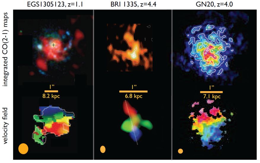
Figure 7. Best examples of resolved molecular line emission at high redshift from which gas kinematics can be derived. These are (from left to right): The CSG EGS 13035123 (Tacconi et al. 2010), the QSO BRI 1335 (Riechers et al. 2008b) and the SMG GN 20 (Hodge et al. 2012). The top row shows the integrated CO(2–1) maps of the targets. The bottom row shows the velocity fields of the targets; here the color indicates the velocity at which gas is moving a given position on the sky. The velocity scale ranges from (blue to red): –65 to +100 km s−1, –154 to +154 km s−1, –300 to 300 km s−1, respectively. The beamsizes are given in the bottom left of each galaxy; the bar indicates 1" on the sky (size in kpc is also given at the respective redshift).

4.6.1. A typical CSG In their ground breaking studies of CSG, Tacconi et al. (2010) and Daddi et al (2010a) find gas rich disks without extreme starbursts (see also Tacconi et al. 2012; Sec. 3.5). The best imaging study to date of a CSG is that of the CO(3–2) emission from EGS 13035123 using the PdBI at 0.6" resolution by Tacconi et al. (2010) (Fig. 7). The H₂ mass is 1.3 × 10¹¹ (α / 3.2) M_⊙, distributed in a rotating disk with a radius of 8 kpc, and a terminal rotation velocity of 200 km s⁻¹. While clearly rotating, the disk also has a high internal velocity dispersion ≥ 20 km s⁻¹, implying substantial disk turbulence.

The disk is punctuated by high brightness temperature clumps with radii ≤ 2 kpc and masses ∼ 5 × 10⁹ M_⊙. The gas surface densities are ∼ 500 M_⊙ pc⁻², a factor few larger than for Galactic GMCs, and they hypothesize that these clumps are conglomerates of a number of Galactic–type GMCs rather than a single giant GMC, due to the relatively low internal velocity dispersions ( ∼ 20 km s⁻¹) Daddi et al. (2010a) obtain similar imaging results for a few CSG at z ∼ 1.5, although at somewhat lower spatial resolution.

These imaging observations of CO in z ∼ 1 to 3 CSG have been critical to the interpretation that the CSG are gas–dominated, rotating disk galaxies undergoing steady, high levels of star formation (see Sec. 3.5). They also helped to constrain the conversion factor α for these systems through dynamical arguments (Sec. 4.2).

4.6.2. BRI 1335-0417: tidally disturbed gas surrounding a luminous quasar BRI 1335-0417 at z = 4.4 was among the first optically selected, very high–z quasars to be identified with a hyper–luminous FIR host galaxy, implying an accreting SMBH with mass ∼ 10⁹ M_⊙ coeval with an extreme starburst (SFR ∼ 1000 M_⊙ yr⁻¹) (Guilloteau et al. 1997). The host galaxy has been detected in CO line emission, with an implied M(H₂) ∼ 8 × 10¹⁰(α / 0.8) M_⊙ (Carilli et al. 2002a), as well as strong [C II] emission (Wagg et al. 2010). BRI 1335-0417 is a broad absorption line quasar, indicating AGN outflow. Fig. 7 (middle) shows the CO images from the of BRI 1335-0417 from the VLA (Riechers et al. 2008b). These are the highest quality CO images of any non–lensed high–z quasar to date. The system shows complex morphology in the gas on a scale of ∼ 1″. The molecular gas shows multiple components distributed over ∼ 7 kpc, with a pronounced tail extending to the north, peaking in a major CO clump ∼ 0.7″ from the quasar, and with a few other streams connecting to the quasar from other directions. While there is an overall north–south velocity gradient, the general velocity field appears chaotic.

Riechers et al. interpret the complex gas structure in BRI 1335-0417 as tidal remnants from a late–stage, gas–rich (‘wet') merger. The merger drives gas accretion onto the main galaxy, fueling the hyper–starburst and the luminous AGN, generally consistent with the high molecular excitation seen in quasar hosts (Sec. 4.1). For comparison, the SMG–quasar pair BRI 1202-0725 at z ∼ 4.7 shows a distinct SMG and quasar, possibly corresponding to an early–stage merger, before galaxy coalesence (Salome et al. 2012, Carilli et al. 2012).

4.6.3. GN 20: an SMG with a gas rich disk The galaxy GN 20 is the brightest SMG in the GOODS–North field (Pope et al. 2006), and the host galaxy is heavily obscured at optical wavelengths. Daddi et al. (2009a) made a serendipitous redshift determination of z = 4.05 from CO emission using the PdBI (by targeting a nearby CSG). Two other SMGs at this redshift have been detected in CO and dust continuum emission about 20" to the west (Carilli et al. 2011; Hodge et al. 2012), and there is a clear over–density of galaxies in this field, with 15 LBGs with z_phot ∼ 4 within a radius or 25" of GN 20 (Daddi et al. 2009).

A long observation using the JVLA in early science of the CO (2–1) emission (Hodge et al. 2012) shows that the CO is distributed in a disk with a diameter ∼ 14 kpc (Fig. 7, right). The regions emitting in CO and dust continuum are mostly obscured in the HST I–band image. The only tracable optical emission is seen at the edges of the source (Hodge et al. 2012). Such heavy obscuration in the optical is characteristic of SMGs.

The GN 20 disk dynamics are consistent with a standard ‘tilted–ring' gas rotation model, with a dynamical mass of 5.4 ± 2.4 10¹¹ M_⊙. Observations at 1kpc resolution reveal that 30% to 50% of the gas is in giant clumps with gas masses of a few × 10⁹ (α / 0.8) M_⊙, brightness temperatures between 16 K and 31 K, and line widths of order 100 km s⁻¹ (Hodge et al. 2012). A dynamical analysis suggests the clumps could be self–gravitating. The gas surface densities of the clumps are ∼ 4000 (α / 0.8) M_⊙ pc⁻², more than an order of magnitude larger than typical GMCs. An analysis of the overall galaxy dynamics has been used to determine the value of α in GN 20 (see Sec. 4.2).

The apparent disk in GN 20 suggests that not all HyLIRGs at very high redshift result from an ongoing major merger. This conclusion has also been reached for a few other SMGs at lower redshift, where low order CO observations show large, disk–like gas reservoirs similar to GN 20 (Ivison et al. 2011; Riechers et al. 2011; Greve et al. 2004, Ivison et al. 2010a, b).

In GN 20, the clumpy disk is consistent with that expected in the cold mode accretion model (e.g. Kereš et al. 2005, Dekel et al. 2006, 2009), only now scaled up by almost an order of magnitude in FIR luminosity relative to typical CSG (Sec. 5.1.2). It is possible that the star formation in this gas rich disk has been enhanced due to gravitational harrasment by the other SMGs and smaller galaxies in the proto–cluster.

Spatially resolving the molecular gas emission in high redshift galaxies is to date restricted to very few, bright, sources. Imaging the molecular and cool atomic gas a few selected high redshift galaxies has revealed 10 kpc–scale, clumpy and turbulent, but apparently rotating disks in CSG and some SMGs, as well as strongly tidally disturbed gas distributions in some SMGs and quasar hosts.

4.7. Outflows

Theoretical models without negative feedback (negative feedback = ejection of material due to either star formation or AGN activity) predict both a higher gas content in massive galaxies in the nearby Universe, and a larger population of star forming massive galaxies today, than observed. At high galactic masses, including AGN feedback mitigate these problems in simulations, both driving gas out of the immediate ISM of the host galaxy via AGN winds, and suppressing further gas accretion from the IGM via large–scale radio jets (Fabian 2012). Direct evidence for feedback has been seen in nearby galaxies, including outflows seen in OH far–IR lines, molecular emission lines, optical lines, and atomic fine structure lines (e.g., in the case of M 82: Strickland & Heckman 2009, Walter et al. 2002, Martin 1998). The fact that old, gas–poor massive galaxies have now been seen at redshifts of 2 and beyond suggest that feedback must be an important process even earlier.

Recent observations have detected evidence for feedback on kpc–scales in very early galaxies. One of the best examples of AGN feed–back are the broad line wings of the [C II] emission from the z = 6.4 quasar J1148+5251 by Maiolino et al. (2012). They derive an outflow velocities of 1300 km s⁻¹, an outflow rate of _outfl ∼ 3500 M_⊙ yr⁻¹, and kinetic power of: P_K ∼ 1.9 × 10⁴⁵ erg s⁻¹. This is roughly 0.6% of the quasar bolometric luminosity, well below the theoretical upper limit to a radiatively driven quasar outflow of 5% of the bolometric luminosity (Lapi et al. 2005), but it is barely consistent with the maximum kinetic power that can be driven by the associated starburst in the quasar host (Veilleux et al. 2005). Likewise, theoretical models indicate that star formation driven winds reach a maximum velocity of ∼ 600 km s⁻¹ (Thacker et al. 2006). Maiolino et al. (2012) argue that the outflow is most likely AGN–driven. The gas consumption timescale for the outflow is comparable to that due to star formation, of order 10⁷ yr.

Other systems show varying degrees of feedback in the cooler gas. The BRI 1202-0725 quasar–SMG galaxy pair does show evidence for a broad wing in the quasar host galaxy [C II] 158µm spectrum, but the outflow kinetic energy is well below that of J1148+5251, and star formation likely dominates gas depletion in the galaxy (Wagg et al. 2012; Carilli et al. 2012). Weiß et al. (2012) detect a 250 km s⁻¹ outflow in a z = 2.8 quasar in both CO and [C I]. They derive a lower limit to the mass outflow rate of 180 M_⊙ yr⁻¹, which is slightly larger than the star formation rate in the host galaxy.

Molecular Outflows have only very recently been detected in a few high–redshift systems. Given that they feature (by definition) broad and faint line wings they remained undetected by past observations, both due to missing sensitivity and insufficient bandwidth. Quantifying the kinetic energy and masses associated with such outflows will provide important input in galaxy simulations in which feedback by stellar (or AGN) activity is a key driver for galaxy evolution.

¹ Including a correction for the relative contribution of the CMB increases these values by about 35% at z = 2.5 (Ivison et al. 2011). Back.