


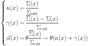
In most cases, intermediate redshift z ∼ 0.2 − 0.5 massive clusters are the most significant mass distribution along the line of sight, thus they can be represented by a single lens plane in concordance with the thin lens approximation. In the ΛCDM model, the probability of finding two massive clusters extremely well aligned along the line of sight (albeit separated in redshift) is extremely unlikely as clusters are very rare objects. Lensing deflections and distortions probe the two dimensional projected cluster mass along the line of sight. This allows us to constrain the two dimensional Newtonian potential, φ(x, y), resulting from the three-dimensional density distribution ρ(x, y, z) projected onto the lens plane. The related projected surface mass density Σ(x, y) is then given by:
 |
(42) |
Often we are interested in the two-dimensional projected mass inside an aperture radius R (particularly when comparing different mass estimators), which is defined explicitly as follows:
 |
(43) |
and the mean surface density inside the radius R is given by:
 |
(44) |
The important quantities for lensing in clusters are primarily
the deflection angle
 between
the image and the source, the convergence κ, and the shear
γ, which can all be conveniently expressed in terms of the
projected potential:
between
the image and the source, the convergence κ, and the shear
γ, which can all be conveniently expressed in terms of the
projected potential:
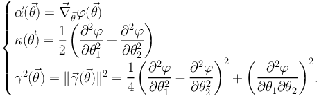 |
(45) |
For a radially symmetric mass distribution, these expressions can be written as:
 |
(46) |
where x = DOL θ is the radial physical distance. From this equation, we note that one can derive γ directly from α and κ. This formulation is particularly useful when trying to compute an analytic expression of the lensing produced by a given mass profile.
Traditionally, modeling of the cluster mass distribution in the strong lensing regime is done using “parametric models” (e.g. Kneib et al. 1996; Natarajan & Kneib 1997). In these schemes the mass distribution is described by a finite number of mass clumps; some small scale (galaxy components) and some large scale (to represent the dark matter, X-ray gas in the Intra-Cluster Medium), each of which are described in turn by a finite number of parameters contingent upon the choice of mass profile deployed. The simplest mass distribution that is commonly employed is the circular Singular Isothermal Sphere (SIS), which is described by three parameters. The parameters are the position of its center (x, y) and the value of the velocity dispersion σ, which in this case is a constant. Other mass distributions such as the PIEMD (Pseudo Isothermal Elliptical Mass Distribution) or NFW (Navarro-Frenk-White) profiles are often used in lensing analysis and their relevant parameters are described in the Appendix (see A.1 - A.3).
Using a simple mass model makes sense when there are not many available observational constraints indeed one needs to balance the number of model parameters to the number of observational constraints available in order to compute a sensible best-fit model. However, with recent deep images of cluster cores from HST a very large number of multiple-images can readily be identified. For instance, more than 40 multiple-image systems have been identified in the massive cluster Abell 1689 by Limousin et al. (2007). The discovery and identification of such a large number of multiple-images has dramatically increased the number of constraints available for mass modeling of massive clusters in the last decade. With the availability of a larger number of multiply imaged systems with redshift measurements, more accurate mass models (Figure 18) are now possible.
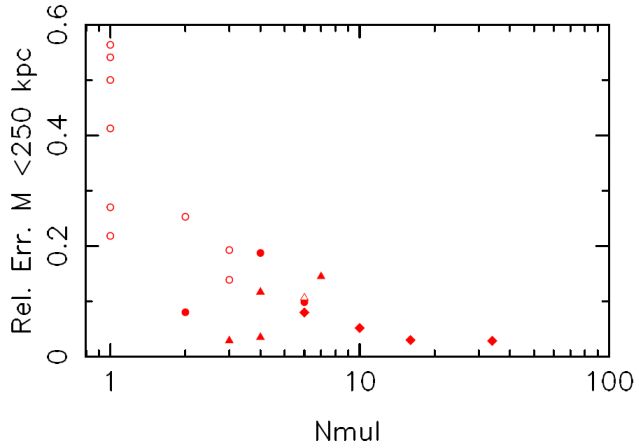 |
Figure 18. Relative aperture mass error as a function of the number of multiple-images as measured in Richard et al. (2010). Open symbols: clusters observed with WFPC2. Filled symbols: clusters observed with ACS. Symbols reflect the number of filters used to image the cluster (circle: 1 filter, triangle: 2 filters, diamond: 3 or more filters). One can see that with multi-band ACS data we can uncover more than 10 multiple-image systems for the most massive clusters, and thus achieve mass accuracy within 10% or so in cluster cores. |
Therefore, the number of allowable parameters required to describe the mass distribution of a cluster has also increased, leading obviously to a more accurate description of the mass profile in the cluster core. This is for example evident upon comparing the model of Kneib et al. (1993) with that of Richard et al. (2010) for the cluster Abell 370. In the case of “parametric models”, the increase in the number of constraints translates to the fact that cluster mass distributions can now be described by a larger number of mass clumps and each of these clumps can be more complex (e.g. having elliptical mass distributions rather than circular, and a radial profile described by more parameters).
The increase in the number of available constraints has also lead to the development of new “non-parametric” methods, where no (or few) external priors are required to describe the mass distribution of clusters (Diego et al. 2005a; Saha & Williams 1997; Coe et al. 2010). Generically, in most of these 'non-parametric' methods, the mass distribution is typically tessellated into a regular grid of smaller mass elements. Further details of such methods are discussed later on in this section.
3.1.2. From simple to more complex mass determinations
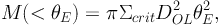
A particularly useful and popular mass estimate in the strong lensing regime is the mass enclosed within the Einstein radius θE, given by:
 |
(47) |
where θE is the location of the tangential critical line for a circular mass distribution, usually approximated by the tangential arc radius θarc. It is a very handy expression that is independent of the mass profile for circularly symmetric cases. However, caution needs to be exercised when using this expression as often the arc used to derive the mass has an unknown redshift (thus Σcrit is not well defined), or the arc is a single image and therefore does not trace the Einstein radius or the mass distribution is very complex with a lot of substructure. Note that, however, for a singular isothermal sphere model, a single image cannot be closer than twice the Einstein radius since it will then have a counter image. In conclusion, this estimator tends to typically overestimate the mass in instances where the tangential arc is not multiply imaged or its redshift is unknown.
The radial critical line can be constrained when a radial arc is observed in the cluster core, this has now been done for a number of cluster lenses (e.g. Fort et al. 1992; Smith et al. 2001; Sand et al. 2002; Gavazzi et al. 2003). These features are important as they lie very close to the cluster core, and thus provide a unique probe of the surface mass density in the very center. Baryons are highly concentrated in the inner regions of clusters and they are expected to play an important role in possibly modifying the dark matter distribution on the smallest scales. The scales on which these effects are expected are accessible effectively with lensing data. Radial arcs have been used to probe the dark matter slope in the inner most regions of clusters (Sand et al. 2005, 2008; Newman et al. 2011), the results of these studies will be discussed in detail later on in this review.
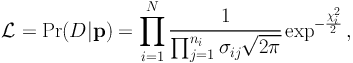
The proper way to accurately constrain the mass in cluster cores is thus to use multiple-images with preferably measured spectroscopic redshifts to absolutely calibrate the mass. To do this, one generally defines a likelihood L for the observed data D and parameters p of the model:
 |
(48) |
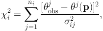
where N is the number of systems, and ni the number of multiple-images for the system i. The contribution from the multiple-image system i to the overall χ2 can be simply given by:
 |
(49) |
where θj(p) is the position of image j predicted by the current model, whose parameters are p and where σij is the error on the position of image j.
The accurate determination of σij depends on the signal-to-noise of the image S/N ratio. For extended images, a pixellated approach is the only accurate way to take the S/N ratio of each pixel into account (Dye & Warren 2005; Suyu et al. 2006) but this is not optimal for cluster lenses with a large number of multiple-image systems. However, to a first approximation, the positional error of images can be determined by fitting a 2D Gaussian profile to the image surface brightness, which assumes that the background galaxy is compact and its surface brightness profile is smooth enough so that the brightest point in the source plane can be reliably matched to the brightest point in the image plane.
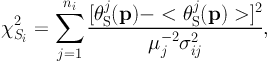
A major issue in the χ2 computation is how to match the predicted and observed images one by one. In models producing different configurations of multiple-images (e.g. a radial system instead of a tangential system), the χ2 computation will fail and the corresponding model will then be rejected. This usually happens when the model is not yet well determined, and this can slow down the convergence of the modeling significantly. To get around this complexity, one often computes the χ2 in the source plane (by computing the difference in the source position for a given parameter sample p) instead of doing so in the image plane. The source plane χ2 is written as:
 |
(50) |
where θSj(p) is the corresponding source position of the observed image j, < θSj(p) > is the barycenter position of all the ni source positions, and µj is the magnification for image j. Written in this way, there is no need to solve the lensing equation repeatedly and so the calculation of the χ2 is very fast. However, in the case where only a small number of multiple-image systems are used, source plane optimization may lead to a biased solution, typically favoring mass models with large ellipticity.
It is important to use physically well motivated representations of the mass distribution and adjust these in order to best reproduce the different families of observed multiple images (e.g. Kneib et al. 1996; Smith et al. 2001) iteratively. Indeed, once a set of multiple-images is securely identified, other multiple-image systems can in turn be discovered using morphological/color/redshift-photometric criteria, or on the basis of the lens model predictions. Better data, or data at different wavelengths may also bring new information enabling new multiple-images to be identified increasing the number of constraints for modeling and hence the accuracy of mass models.
3.1.3. Modeling the various cluster mass components
In a cluster, the positions of multiple-images are known to great accuracy and they are usually scattered at different locations within the cluster inner regions. A simple mass model with one clump cannot usually successfully reproduce observed image configurations.
We know that galaxies in general are more massive than represented by their stellar content alone. In fact, the visible stellar-mass represents only a small portion (likely 10 - 20%) of their total mass. The existence of an extended dark matter halo around individual galaxies has been established for disk galaxies with the measurement of their flat and spatially extended rotation curves (e.g. van Albada et al. 1985). The existence of a dark matter halo has been accepted for ellipticals only relatively recently (e.g. Kochanek et al. 1995; Rix et al. 1997). These studies found that while the stellar content dominates the central parts of galaxies, at distances larger than the effective radius the dark matter halo dominates the total mass inventory. What is less obvious in clusters of galaxies, given their dense environments, is how far the dark halos of individual early-type galaxies extend. One expects tidal“stripping” of extended dark matter halos to occur as cluster galaxies fall in and traverse through cluster cores during the assembly process. This is borne out qualitatively by the strong morphological evolution observed in cluster galaxies (e.g. Lewis, Smail & Couch 2000; Kodama et al. 2002; Treu et al. 2003). In fact, lensing offers a unique probe of the mass distribution on these smaller scales within cluster environments.
The lensing effects of individual galaxies in clusters was first noted by Kassiola et al. (1992) who detected that the lengths of the triple arc in Cl0024+1654 can only be explained if the galaxies near the ‘B' image were massive enough. Detailed treatment of the individual galaxy contribution to the overall cluster mass distribution became critical with the refurbishment of the HST as first shown by Kneib et al. (1996). It was found that cluster member galaxies and their associated individual dark matter halos need to be taken into account to accurately model the observed strong lensing features in the core of Abell 2218.
The theory of what is now referred to as galaxy-galaxy lensing in clusters was first formulated and discussed in detail by Natarajan & Kneib (1997), and its application to data followed shortly (Natarajan et al. 1998; and Geiger & Schneider 1999). From their detailed analysis of the cluster AC114, Natarajan et al. (1998) concluded that dark matter distributed on galaxy-scales in the form of halos of cluster members contributes about 10% of the total cluster mass. Analysis of this effect in several cluster lenses at various redshifts seems to indicate that tidal stripping does in fact severely truncate the dark matter halos of infalling cluster galaxies. The dark matter halos of early-type galaxies in clusters is found to be truncated compared to that of equivalent luminosity field galaxies (Natarajan et al. 2002, 2004). More recent work finds that tidal stripping is on average more efficient for late-type galaxies compared to early-type galaxies (Natarajan et al. 2009) in the cluster environment.
Lens models need to include the contribution of small scale potentials in clusters like those associated with individual cluster galaxies to reproduce the observed image configurations and positions. As there are only a finite number of multiple-images, the number of constraints is limited. It is therefore important to limit the number of free parameters of the model and keep it physically motivated – as in the end – we are interested in deriving physical properties that characterize the cluster fully.
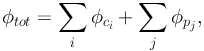
Generally, in these parametric approaches, the cluster gravitational potential is decomposed in the following manner:
 |
(51) |
where we distinguish smooth, large-scale potentials φci, and the sub-halo potentials φpj that are associated with the halos of individual cluster galaxies as providing small perturbations (Natarajan & Kneib 1997). The smooth cluster-scale halos usually represent both the dark matter and the intra-cluster gas. However, combining with X-ray observations, each of these two components could in principle be modeled separately. For complex systems, more than one cluster-scale halo is often needed to fit the data. In fact, this is the case for many clusters: Abell 370, 1689, 2218 to name a few.
The galaxy-scale halos included in the model represent all the massive cluster member galaxies that are roughly within two times the Einstein radius of the cluster. This is generally achieved by selecting galaxies within the cluster red sequence and picking the brighter ones such that their lensing deflection is comparable to the spatial resolution of the lensing observation. Studies of galaxy-galaxy lensing in the field have shown that a strong correlation exists between the light and the mass profiles of elliptical galaxies (Mandelbaum et al. 2006). Consequently, to a first approximation, in mass modeling the location, ellipticity and orientation of the smaller galaxy halos are matched to their luminous counterparts.
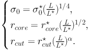
Except for a few galaxy-scale sub-halos that do perturb the locations of multiple-images in their vicinity or alter the multiplicity of lensed images in rare cases, the vast majority of galaxy-scale sub-halos act to merely increase the total mass enclosed within the Einstein radius. In order to reduce the number of parameters required to describe galaxy-scale halos, well motivated scaling relations with luminosity are often adopted. Following the work of Brainerd et al. (1996) for galaxy-galaxy lensing in the field, galaxy-scale sub-halos within clusters are usually modeled with individual PIEMD potentials. The mass profile parameters for this model are the core radius (rcore), cut-off radius (rcut), and central velocity dispersion (σ0), which are scaled to the galaxy luminosity L in the following way:
 |
(52) |
The total mass of a galaxy-scale sub-halo then scales as (Natarajan & Kneib 1997):
 |
(53) |
where L⋆ is the typical luminosity of a galaxy at the cluster redshift. When r⋆core vanishes, the potential becomes a singular isothermal potential truncated at the cut-off radius.
In the above scaling relations (Equation 52), the velocity dispersion scales with the total luminosity in agreement with the empirically derived Faber-Jackson relations for elliptical galaxies (for spiral galaxies the Tully-Fisher should be used instead, but those are not numerous in cluster cores). When α = 0.5, the mass-to-light ratio is constant and is independent of the galaxy luminosity, however, if α = 0.8, the mass-to-light ratio scales with L0.3 similar to the scaling seen in the fundamental plane (Jorgensen et al. 1996; Halkola et al. 2006). Other scalings are of course permissible, and a particularly interesting one that has been recently explored in field galaxy-galaxy lensing studies, is to scale the sub-halo mass distribution directly with the stellar-mass (see Leauthaud et al. 2011).
State of the art parametric modeling is done in the context of a fully Bayesian framework (Jullo et al. 2007), where the prior is well defined and the marginalization is done over all the relevant model parameters that represent the cluster mass distribution. Indeed, the Bayesian approach is better suited than regression techniques in situations where the data by themselves do not sufficiently constrain the model. In this case, prior knowledge about the Probability Density Function (PDF) of parameters helps to reduce degeneracies in the model. The Bayesian approach is well-suited to strong lens modeling given the few constraints generally available to optimize a model. The Bayesian approach provides two levels of inference rather efficiently: parameter space exploration, and model comparison. Bayes Theorem can be written as:
 |
(54) |
where Pr(p|D, M) is the posterior PDF, Pr(D|p, M) is the likelihood of getting the observed data D given the parameters p of the model M, Pr(p|M) is the prior PDF for the parameters, and Pr(D|M) is the evidence.
The value of the posterior PDF will be the highest for the set of parameters p which gives the best-fit and that is consistent with the prior PDF, regardless of the complexity of the model M. Meanwhile, the evidence Pr(D|M) is the probability of getting the data D given the assumed model M. It measures the complexity of model M, and, when used in model selection, it acts as Occam's razor. 5
Jullo et al. (2007) have implemented in Lenstool 6 a model optimization based on a Bayesian Markov Chain Monte Carlo (MCMC) approach, which is currently widely used. Since this approach involves marginalizing over all relevant parameters, it offers a clearer picture of all the model degeneracies.
3.2. Probing the radial profile of the mass in cluster cores
One important prediction from dark matter only numerical simulations of structure formation and evolution in a ΛCDM Universe, is the value of the slope β of the density profile ρdark matter∝ r−β in the central part of relaxed gravitational systems. Although there has been ongoing debate for the past decade on the exact value of the inner slope (Navarro, Frenk & White 1997 (β = 1); Moore et al. 1998 (β = 1.5)), the real limitation of such predictions is the lack of baryonic matter in these simulations. Baryons dominate the mass budget and the gravitational potential in the inner most regions of clusters and need to be taken into account while trying to constrain the inner slope of the dark matter density profile. This is expected to change in the near future with better numerical simulations. Even in dark matter only simulations, it has been found that non-singular three-parameter models, e.g. the Einasto profile has a better performance than the singular two-parameter NFW model in the fitting of a wide range of dark matter halo structures (Navarro et al. 2010). Nevertheless, the radial slope of the total mass profile is a quantity that lensing observations can uniquely constrain (e.g. Miralda-Escude 1995). This was first attempted for Abell 2218 by Natarajan & Kneib (1996) and subsequently by Smith et al. (2001) for the cluster Abell 383, by modeling the cluster center as the sum of a cD halo and a large-scale cluster component. Abell 383 is an interesting and unique system wherein both a tangential and a radial arc with similar redshift are observed. Such a configuration provides a particularly good handle on the inner slope (here considered as the sum of the stellar and Dark Matter component), which in the case of Abell 383 was found to be steeper than the NFW prediction.
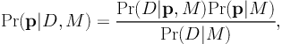
Once tangential and radial arcs have been identified from HST images (see Figure 19), the main observational limitation is the measurement of the redshift of the multiply imaged arc to firmly constrain the radial mass profile. Large telescopes (Keck/VLT/Gemini/Subaru) have been playing a key role in cluster lensing by measuring the redshifts of multiple-images. Furthermore, working at high spectral resolution allows one to also probe the dynamics of cD galaxies in the core of clusters (Natarajan & Kneib 1996; Sand et al. 2002). Thus combining constraints from stellar dynamics, in particular, measurements of the velocity dispersion of stars and coupling that with lensing enables the determination of the mass distribution in cluster cores. This combination is very powerful as it weighs the different mass components individually: stellar-mass, X-ray gas and dark matter in the cores of clusters. Sand et al. (2005) applied this technique to the clusters MS2137-23 and Abell 383 and found that the dark matter component is best described by a generalized NFW model with an inner slope that is shallower than the theoretically predicted canonical NFW profile. A similar analysis was also conducted by Gavazzi et al. (2003) with the same result. It must be stressed that the comparison between numerical simulations and observations is not direct as the stars in the cD galaxies dominate the total mass budget in the very center and the additional contributions of these baryons are not accounted for in the dark matter only simulations. It is widely believed that the significant presence of baryons in cluster cores likely modifies the inner density profile slope of dark matter, although there is disagreement at present on how significant this adiabatic compression is likely to be (Blumenthal et al. 1986; Gnedin et al. 2004; Zappacosta et al. 2006). Radial arcs offer a unique and possible only handle to probe the inner slopes of density profiles. Several other clusters with radial arcs have been discovered from HST archives recently, and are currently being followed up spectroscopically (Sand et al. 2005, 2008).
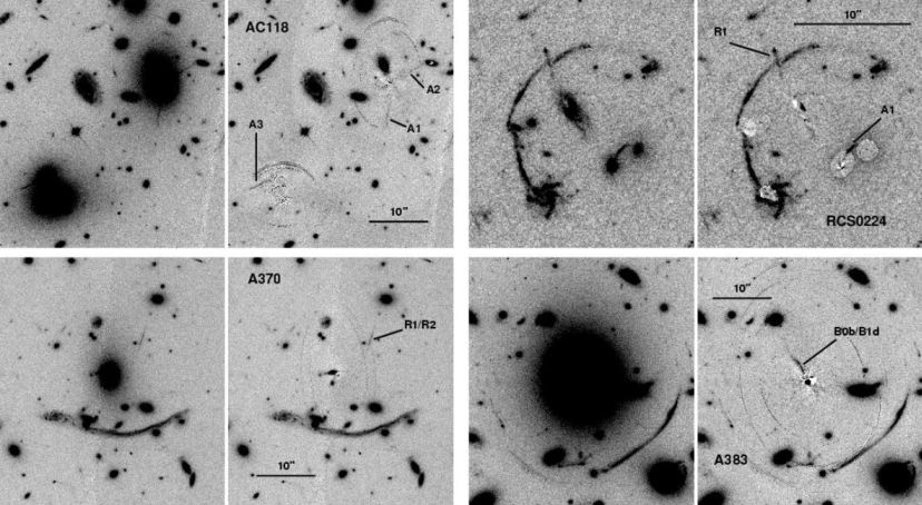 |
Figure 19. Example of radial arcs found in the 4 cluster AC118, RCS0224, A370 and A383 (from Sand et al. 2005). The right side of each panel shows the BCG subtracted images. |
In a recent paper, Newman et al. (2011) have obtained high accuracy velocity dispersion measurements for the cD galaxy in Abell 383 out to a radius of ∼ 26 kpc for the first time in a lensing cluster. Adopting a triaxial dark matter distribution, an axisymmetric dynamical model and using the constraints from both strong and weak lensing, they demonstrate that the logarithmic slope of the dark matter density at small radii is β < 1.0 (95% confidence), shallower than the NFW prediction (see Figure 20). Similar analysis of other relaxed clusters, including constraints from small to large scales will help improve our understanding of the mass distribution in cluster cores and help test the assumptions used in numerical simulations where both dark matter and baryonic matter (stars and X-ray-gas) are explicitly included.
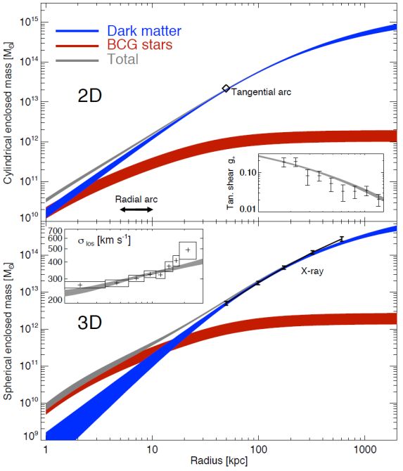 |
Figure 20. Top: Projected mass for the dark matter and stellar components, as well as the total mass distribution, with tangential reduced shear (g) data inset at the same radial scale for the cluster Abell 383. Bottom: 3D Mass, with velocity dispersion data inset and X-ray constraints overlaid. All bands show 68% confidence regions. The models acceptably fit all constraints ranging from the smallest spatial scales ≃ 2 kpc to ≃1.5 Mpc. This figure is taken from Newman et al. (2011). |
3.3. Non-Parametric Strong Lensing modeling
In addition to the use of the parametric analytic mass models described above, there has been considerable progress in developing non-parametric mass reconstruction techniques in the past decade (e.g. Abdelsalam et al. 1998; Saha & Williams 1997; Diego et al. 2005a, b; Jullo & Kneib 2009; Coe et al. 2010; Zitrin et al. 2010). Non-parametric cluster mass reconstruction methods have become more popular with the increase in available observational constraints from the numerous multiple-images that are now more routinely found in deep HST data (e.g. Broadhurst et al. 2005). Non-parametric models have increased flexibility which allows a more comprehensive exploration of allowed mass distributions. These schemes are particularly useful to model extremely complex mass distributions such as the 'Bullet Cluster' (Bradač et al. 2005).
Contrary to the analytic profile driven“parametric” methods, in 'non-parametric' schemes, the mass distribution is generally tessellated into a regular grid of small mass elements, referred often to as pixels (Saha & Williams 1997; Diego et al. 2005a). Alternatively, instead of starting with mass elements, Bradač et al. (2005) prefer tessellating the gravitational potential because its derivatives directly yield the surface density and other important lensing quantities that can be related more straightforwardly to measurements. Pixels can also be replaced by radial basis functions (RBFs) that are real-valued functions with radial symmetry. Several RBFs for density profiles have been tested so far. Liesenborgs et al. (2007) use Plummer profiles, and Diego et al. (2007) use RBFs with Gaussian profiles. The properties of power law profiles, isothermal profiles as well as Legendre and Hermite polynomials have been explored as RBFs. These studies find that the use of compact profiles such as the Gaussian or Power law profiles are generally preferred as they are more accurate in reproducing the surface mass density.
In more recent work, instead of using a regular grid, Coe et al. (2008, 2010) and Deb et al. (2008) use the actual distribution of images as an irregular grid. Then, they either place RBFs on this grid or directly estimate the derivatives of the potential at the location of the images. Whatever their implementation, the reproduction of multiple-images is generally greatly improved with respect to traditional 'parametric' modeling with these techniques. However, the robustness of these models is still a matter of debate given the current observational constraints available from data. Indeed, due to the large amount of freedom that inevitably goes with the large degree of flexibility afforded by a “non-parametric” approach, many models can fit perfectly the data and discriminating between models is challenging. To identify the best physically motivated model and eventually learn more about the dark matter distribution in galaxy clusters, additional external criteria (e.g. mass positivity) or regularization terms (e.g. to avoid unwanted high spatial frequencies) are necessary. Furthermore, galaxy mass scales are usually not taken into account in these non-parametric schemes, despite the fact that successful parametric modeling has clearly demonstrated that these smaller scale mass clumps do significantly affect the positions of observed multiple-images. This is a key limitation of most of the 'non-parametric' models.
Jullo & Kneib (2009) [JK09 hereafter] have proposed a novel modeling scheme that includes both a multi-scale grid of RBFs and a sample of analytically defined galaxy-scale dark matter halos, thus allowing combined modeling of both complex large-scale mass components and galaxy-scale halos. In this hybrid scheme, similar to the one adopted by Diego et al. (2005a), JK09 define a coarse multi-scale grid from a pixelated input mass map and recursively refine it in the densest regions. However, in contrast to previous work, they start from a hexagonal grid (composed of triangles), on the grounds that it better fits the generally roundish shapes of galaxy clusters. For their RBF, they use truncated circular isothermal mass models, and truncated PIEMD models to explicitly include galaxy-scale halos. Thus both components are modeled with similar analytical functions which permits a simple combination for ready incorporation into the Bayesian MCMC optimization scheme built into LENSTOOL. Figure 21 shows the derived S/N convergence map for the model of the cluster A1689. As the S/N of the mass reconstruction is found to be larger than 10 everywhere inside the hexagon, the error in the convergence derived mass is less than 10%, demonstrating the power of this hybrid scheme.
 |
Figure 21. Map of S/N ratio for the A1689 mass reconstruction using the JK09 "non-parametric" mass reconstruction. Colored contours bound regions with S/N greater than 300, 200, 100 and 10. The highest S/N region is at the center where there are the most constraints. Red contours are mean iso-mass contours. Black boxes mark the positions of the multiple-images used to constrain the mass distribution, and the numbers indicate the di erent multiple-image systems (from JK09). |
3.4. Cluster Weak lensing modeling
As soon as we look a little bit further out radially from the cluster core, the lensing distortion gets smaller (distortions in shape get to be of the order of a few percent at most), and very quickly the shape of faint galaxies gets dominated by their intrinsic ellipticities (the dispersion of the intrinsic ellipticity distribution of observed galaxies σє ∼ 0.25). Thus the lensing distortion is no longer visible in individual images and can only be probed in a statistical fashion, characteristic of the weak lensing regime (e.g. Bartelmann 1995). The nature of constraints provided by observations are fundamentally different in the weak lensing regime compared to the strong lensing regime. In the strong regime, as we shown above every set of observed multiple-images provides strong constraints on the mass distribution. In the weak regime, however, what is measured are the mean ellipticities and/or the mean number density of faint galaxies in the frame. In order to relate these to the mean surface mass density κ of the cluster, these data need to be used statistically. There are two key sets of challenges in doing so:
• Observational : How to best determine the ‘true' ellipticity of an observed faint galaxy image which is smeared by a PSF of comparable size, and is not circular (as a result of camera distortions, variable focus across the image, tracking and guiding errors) and not stable in time? How best to estimate and isolate the variation in the number density of faint galaxies due to lensing, while taking into account the crowding effect due to the presence of cluster members and the intrinsic spatial fluctuations in the distribution of galaxies; and the unknown redshift distribution of background sources?
• Theoretical : what is the optimal
method to reconstruct the surface mass density distribution κ (as
a mass map or a radial mass profile) using either the ‘reduced
shear field'  and/or
the amplification?
and/or
the amplification?
Various approaches have been proposed to solve these sets of problems, and two distinct families of methods can be distinguished: direct and inverse methods. We describe them in detail in what follows.
3.4.1. Weak lensing observations
For observers, before any data handling, the first step is to choose the telescope (and instrument) that will minimize the sources of noise in the determination of the ellipticity of faint galaxies. Although HST has the best characteristics in terms of the PSF size, it has a very limited field of view ∼ 10 square arcminutes for the ACS camera. Furthermore, Hubble is “breathing” as it is orbiting around the Earth, which affects the focus of its instruments, and the most recent ACS imaging data appear to be suffering from Charge Transfer Inefficiency (CTI) which needs special post-processing for removal of these instrumental effects (Massey 2010). Although, as we have seen HST is ideal for picking out strong lensing features (e.g. Gioia et al 1998), it is not the most appropriate instrument to probe the large scale distribution of a cluster extending out to and beyond the virial radius. Note however, this limitation becomes less of a problem when observing high-redshift clusters (e.g. Hoekstra et al 2002, Jee et al 2005, Lombardi et al 2005).
On the ground a number of wide-field imaging cameras have been used to conduct weak lensing measurements in cluster fields. The most productive ones in the last decades have been: the CFHT12k camera (e.g. Bardeau et al. 2007, Hoekstra 2007) and the more recent Megacam camera (e.g. Gavazzi & Soucail 2007, Shan et al. 2012) at CFHT, and the Suprimecam on Subaru (e.g. Okabe et al. 2010). However a number of studies have also been done with other instruments, in particular, the VLT/FORS (e.g. Cypriano et al. 2001, Clowe et al. 2004), 2.2m/WFI (e.g. Clowe & Schneider 2002), and more recently with the LBT camera (Romano et al. 2010).
3.4.2. Galaxy shape measurement
Once the data have been carefully taken either from the ground or space with utmost care to minimize contaminating distortions and hopefully under the best seeing conditions, the next step is to convert the image of the cluster into a catalog where the PSF corrected shapes of galaxies are computed.
Before measuring the galaxy shape a number of steps are usually undertaken: 1) masking of the data and identifying the regions in the image that suffer from observational defects: bleeding stars, satellite tracks, hot pixels, spurious reflections; 2) source identification and catalog production which is usually done using the Sextractor software (Bertin & Arnouts 1996); 3) identification of the stellar objects in order to accurately compute the PSF as a function of position in the image. Once this is done, the shapes of the stellar objects and galaxies can be computed to derive the PSF corrected shapes of galaxies which will then be used for weak lensing measurements. For accomplishing this crucial next step, a popular and direct approach is often used, to convert galaxy shapes to shear measurements using the Imcat software package. This implementation is based on the Kaiser, Squires and Broadhurst (1995) methodology, but has been subsequently improved by various other groups (e.g. Luppino & Kaiser 1997; Rhodes et al. 2000; Hoekstra et al. 2000), providing variants of the original KSB technique. To correct the galaxy shape from the PSF anisotropy and circularization, the KSB technique uses the weighted moment of the object's surface brightness to find its center, and shape to measure higher order components that can be used to improve the PSF correction. As a result the correction is fast and processing a large amount of data can be done swiftly and efficiently.
Alternatively, one can use the inverse approach using maximum likelihood methods or Bayesian techniques to find the optimal galaxy shape that when convolved with the local PSF best reproduces the observed galaxy shape (e.g. Kuijken, 1999; Im2Shape: Bridle et al. 2002). A recent implementation of this inverse method is available in the Lensfit software package (Miller et al. 2007; Kitching et al. 2008) and one of its key advantages is that it works directly on the individual exposures of a given field. Lensfit has been developed in the context of the CFHT-LS survey, but is flexible and can be easily adapted for use with other observations.
These inverse approaches have the advantage that they provide a direct estimate of the uncertainty in the parameter recovery as illustrated in Figure 22. Further extension of these inverse techniques, has led to the use of Shapelets (Refregier 2003; Refregier & Bacon 2003) that offer a more sophisticated basis set to characterize the two-dimensional shapes of the PSF and faint galaxies. The versatility of shapelets has made this technique quite popular for lensing measurements. Nevertheless, it has been realized that these different shape measurement recipes need to be tuned, compared and calibrated amongst each other in order to obtain accurate, unbiased and robust shear measurements. This calibration work has been done in the context of various numerical challenges, wherein different research groups measure the shapes of the same set of simulated images as part of STEP (Heymans et al. 2006; Massey et al. 2007); the GREAT08 and GREAT10 challenges (Bridle et al. 2010; Kitching et al. 2011). These challenges have proven to be very useful exercises for the community as they have enabled calibration of the several independent techniques employed to derive shear from observed shapes.
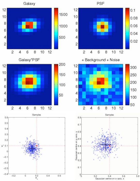 |
Figure 22. Simulated images demonstrating the various sources of noise in weak lensing data: the galaxy model, the PSF model, the convolution of the two, and the final image when noise is added. Simple simulations allow the production of model images that include observational sources of noise and can therefore be compared directly to the shapes of observed faint galaxies. The best galaxy model is then found by taking into account the convolution effect of the measured PSF that best-fits the data. (Bottom panels): the MCMC samples fitting the final image in terms of its ellipticity vector - with coordinates [e+ = e1] and [e × = e2] - (on the left) and in terms of the position (x,y) of the image center (right), from which the best-fit fiducial models with errors can be extracted (black crosses). One of the first implementations of this inverse technique was done in the Im2shape software (Bridle et al. 2002). |
3.4.3. From galaxy shapes to mass maps
From the catalog of shape measurements of faint galaxies, a mass map
can be derived. And here again direct and inverse methods have been
explored. The direct approaches are: (i) the
Kaiser & Squires
(1993)
method - this is an integral method, that expresses κ as the
convolution of  with a kernel and subsequent
refinements thereof (e.g.
Seitz et al. 1995,
1996,
Wilson et al 1996a);
and (ii) a local inversion method
(Kaiser 1995;
Schneider 1995;
Lombardi & Bertin
1998)
that involves the integration of the gradient of
within the boundary of the observed
field to derive κ. This technique is particularly relevant for
datasets that are limited to a small field of view.
with a kernel and subsequent
refinements thereof (e.g.
Seitz et al. 1995,
1996,
Wilson et al 1996a);
and (ii) a local inversion method
(Kaiser 1995;
Schneider 1995;
Lombardi & Bertin
1998)
that involves the integration of the gradient of
within the boundary of the observed
field to derive κ. This technique is particularly relevant for
datasets that are limited to a small field of view.
The inverse approach works for both the κ field and the lensing
potential ϕ and uses a maximum likelihood (e.g.
Bartelmann et al. 1996;
Schneider et al. 2000;
King & Schneider
2001),
maximum entropy method (e.g.
Bridle et al. 1998;
Marshall et al. 2002)
or atomic inference approaches coupled with MCMC optimization
techniques
(Marshall 2006)
to determine the most likely mass distribution (as a 2D mass map or a 1D
mass profile) that reproduces the reduced shear field
and/or the variation in the faint galaxy number
densities. These inverse methods are of great interest as they enable
quantifying the errors in the resultant mass maps or mass estimates
(e.g.
Kneib et al. 2003),
and in principle, can cope with the addition of
further external constraints from strong lensing or X-ray data
simultaneously. Wavelet approaches that use the multi-scale entropy
concept have also been extremely powerful in producing multi-scale mass
maps
(Starck, Pires &
Refregier 2006,
Pires et al 2009).
An important issue for producing mass maps is the resolution at which the 2D lensing mass map can be reconstructed. Generally, mass maps are reconstructed on a fixed size grid, which then automatically defines the minimum mass resolution that can be obtained. By comparing the likelihood of different resolution mass maps, we can calculate the Bayesian evidence of each to determine the optimal resolution (Figure 23). However, it is most likely that the optimal scale to which a mass map can be reconstructed is adaptive, and is determined by the strength of the lensing signal. As we are limited by the width of the intrinsic ellipticity distribution, it is only by averaging over a large number of galaxies that we can reach lower shear levels. Thus low shear levels can only be probed on relatively large scales by averaging over a large number of galaxies. Furthermore, as the projected surface mass density of clusters on large scales falls off relatively quickly scaling as 1/R to 1/R2, respectively, for an SIS or a NFW profile, mass maps may quickly lose spatial resolution.
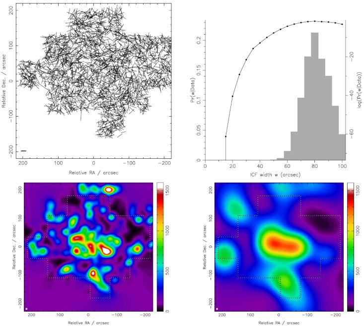 |
Figure 23. Maximum entropy mass reconstruction (Marshall et al. 2002, Marshall 2003) of the X-ray luminous cluster MS1054 at z = 0.83 using Hoekstra's HST dataset (Hoekstra et al. 2000). (Top Left) Distribution of the positions of galaxies used in the mass reconstruction. (Top Right) Evidence values for different sizes of the Intrinsic Correlation Function (ICF). (Bottom) Two mass reconstructions illustrate the case of 2 different values for the ICF: (left) small ICF with a low evidence value, (right) large ICF with the largest evidence. |
Although lensing mass maps may quickly loose information content outside the cluster core, they can be very useful in identifying possible (unexpected) substructures on scales larger than the typical weak lensing smoothing scale (∼ 1 arcminute). This has been the case for several cluster lenses such as the cluster Cl0024+1654 (e.g. Kneib et al. 2003 and Figure 24; Okabe et al. 2009, 2010) and the“Bullet Cluster” (see Figure 25), and more recently in the so-called “baby bullet” cluster (Bradač 2009).
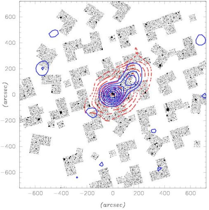 |
Figure 24. The 39 WFPC2/F814W, and the 38 STIS/50CCD pointings sparsely covering the Cl0024+1654 cluster. The (red) dashed contours represent the number density of cluster members as derived by Czoske et al. (2001). The blue solid contour is the mass map built from the joint WFPC2/STIS analysis derived using the LensEnt software (Bridle et al. 1998; Marshall et al. 2002). |
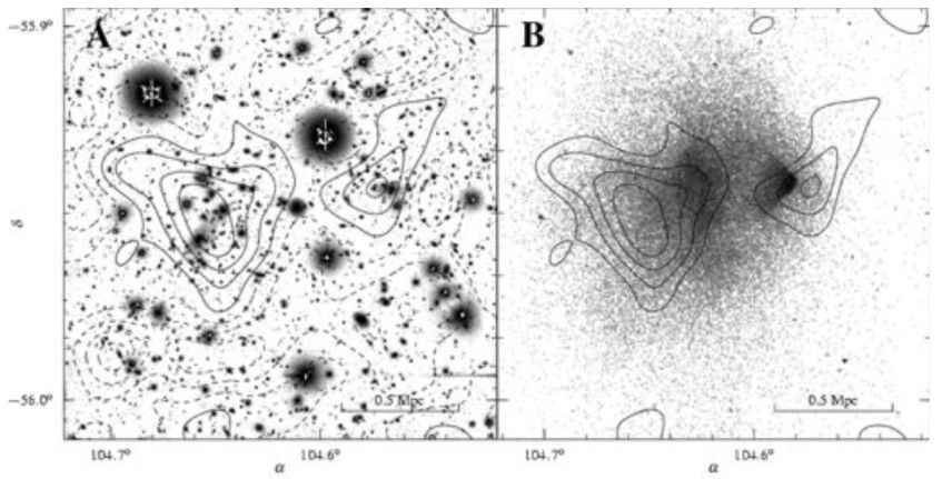 |
Figure 25. Right Panel: Shown in greyscale is the I-band VLT/FORS image of the Bullet cluster used to measure galaxy shapes. Over-plotted in black contours is the weak lensing mass reconstruction with solid contours for positive mass, dashed contours for negative mass, and the dash-dotted contour for the zero-mass level. Left Panel: Shown in greyscale is the Chandra X-ray image from Markevitch et al. (2002) with the same weak lensing contours as in the Right Hand panel. (Figure from Clowe et al. 2004). |
3.4.4. Measuring total mass and mass profiles
Weak lensing mass maps are useful to determine mass peaks, but they are of limited use for the extraction of physical information. If a cluster has a relatively simple geometry (i.e. has a single mass clump in its 2D mass map) one can easily extract the radial mass profile and compute the total mass enclosed within a given radial aperture. Different approaches are currently available to compute the mass profile and the total mass. The direct method is just to sum up the tangential weak shear as expressed in the aperture mass densitometry first introduced by Fahlman et al. (1994) and then revised by Clowe et al. (1998). This statistic is quite popular and has been used in several recent cluster modeling papers, including Hetterscheidt et al. 2004, Hoekstra (2007) and Okabe et al. (2010). Aperture mass densitometry measures the mass interior to a given radius following the ζ statistic, defined as:
 |
(55) |
which provides a lower bound on the mean convergence
 interior to radius θ1.
The mass within θ is then just given by:
interior to radius θ1.
The mass within θ is then just given by:
 |
(56) |
This statistic assumes however that all background galaxies are at a similar redshift, which can be a strong and severely limiting assumption, particularly for high redshift clusters.
Another semi-direct approach is to build the projected surface density contrast ΔΣ estimator as introduced by Mandelbaum et al. (2005):
 |
(57) |
In practice, ΔΣ is measured by averaging over the galaxies at radius r from the cluster center, and requires some information about the redshift distribution of background galaxies zS. It can then be directly compared to the ΔΣ(r) computed for a given parametrized mass model. Mandelbaum et al. (2010) discuss and compare this cluster mass estimator with other proposed ones. In a recent paper, Gruen et al. (2011) compare the use of various aperture mass estimators to calibrate mass-observable relations from weak lensing data.
The alternative method is to directly fit the observables using simple parametric models similar to what is done in the strong lensing approach, for example using radially binned data (e.g. Fischer & Tyson 1997; Clowe & Schneider 2002; King et al 2002; Kneib et al. 2003). The advantage of adopting such a method lies in its flexibility, i.e. allowing combination of strong and weak lensing constraints. This direct approach also allows inclusion of external constraints such as those from X-ray data and the redshift distribution of background sources that can be estimated using photometric-redshift techniques. Of course, such parametric techniques require allowing sufficient freedom in the radial profile and the inclusion of substructures substructures (e.g. Metzler et al. 1999, 2001; King et al. 2001) to closely match observed lensing distortions.
As lensing is sensitive to the integrated mass along the line of sight, it is natural to expect mass overestimates due to fortuitous alignment of mass concentrations not physically related to the cluster or alternatively departures of the cluster dark matter halo from spherical symmetry (e.g. Gavazzi 2005). Till recently, most studies of the dark matter distribution and the intra-cluster medium (ICM) in galaxy clusters using X-ray data have been limited due to the assumption of spherical symmetry. However, the Chandra and XMM-Newton X-ray telescopes have resolved the core of the clusters, and have detected departures from isothermality and spherical symmetry. Evidence for a flattened triaxial dark matter halo around five Abell clusters had been reported early on by Buote & Canizares (1996). Furthermore, numerical simulations of cluster formation and evolution in a cold dark matter dominated Universe do predict that dark matter halos have highly elongated axis ratios (Wang & White 2009), disproving the assumption of spherical geometry. In fact the departures from sphericity of a cluster may help explain the discrepancy observed between cluster masses determined from X-ray and strong lensing observations (Gavazzi 2005). This suggests that clusters with observed prominent strong lensing features are likely to be typically preferentially elongated along the line of sight which might account for their enhanced lensing cross sections. This is definitely the case for the extreme strong lenses with large Einstein radii and therefore anomalously high concentrations. The galaxy cluster A1689 is a well-studied example with such a mass discrepancy (Andersson & Madejski 2004; Lemze et al. 2008; Riemer-Sorensen et al. 2009; Peng et al. 2009). In the same vein, large values of the NFW model concentration parameters have also been reported for clusters with prominent strong lensing features (Comerford & Natarajan 2007; Oguri et al. 2009). This can again be explained by strong lensing cluster halos having their major axis preferentially oriented toward the line of sight (Corless et al. 2009).
Combining strong lensing constraints with high-resolution images of cluster cores in X-rays obtained with Chandra is an excellent way to probe the triaxiality of the mass distribution in cluster cores. Mahdavi et al. (2007) provided a new framework for the joint analysis of cluster observations (JACO) using simultaneous fits to X-ray, Sunyaev-Zel'dovich (SZ), and weak lensing data. Their method fits the mass models simultaneously to all data, provides explicit separation of the gaseous, dark, and stellar components, and allows joint constraints on all measurable physical parameters. The JACO prescription includes additional improvements to previous X-ray techniques, such as the treatment of the cluster termination shock and explicit inclusion of the BCG's stellar-mass profile. Upon application of JACO to the rich galaxy cluster Abell 478 they report excellent agreement among the X-ray, lensing, and SZ data.
Morandi et al. (2010) have used a triaxial halo model for the galaxy cluster MACS J1423.8+2404 to extract reliable information on the 3D shape and physical parameters, by combining X-ray and lensing measurements. They found that this cluster is triaxial with dark matter halo axial ratios 1.53 ± 0.15 and 1.44 ± 0.07 on the plane of the sky and along the line of sight, respectively. They report that such a geometry produces excellent agreement between the X-ray and lensing mass.
These first results are very encouraging and pave the way for a better understanding of the 3D distribution of the various mass constituents in clusters. Theoretically, according to the current dark matter dominated cosmological model for structure formation cluster halo shapes ought to be triaxial and a firm prediction is proffered for the distribution of axis ratios for clusters. More observational work needs to be done to test these predictions, and ultimately techniques that combine lensing, X-ray and Sunyaev-Zel'dovich decrement data might be able to provide a complete 3-dimensional view of clusters.
5 “All things being equal, the simplest solution tends to be the best one.” Back.
6 LENSTOOL is available at - http://lamwws.oamp.fr/lenstool/ Back.