Annu. Rev. Astron. Astrophys. 2017. 55:343-387 Copyright © 2017 by Annual Reviews. All rights reserved

1. INTRODUCTION

Astrophysical observations ranging from the scale of the horizon (∼ 15,000 Mpc) to the typical spacing between galaxies (∼ 1 Mpc) are all consistent with a Universe that was seeded by a nearly scale-invariant fluctuation spectrum and that is dominated today by dark energy (∼ 70 %) and Cold Dark Matter (∼ 25%), with baryons contributing only ∼ 5% to the energy density (Planck Collaboration et al. 2016, Guo et al. 2016). This cosmological model has provided a compelling backbone to galaxy formation theory, a field that is becoming increasingly successful at reproducing the detailed properties of galaxies, including their counts, clustering, colors, morphologies, and evolution over time (Vogelsberger et al. 2014, Schaye et al. 2015). As described in this review, there are observations below the scale of ∼ 1 Mpc that have proven more problematic to understand in the ΛCDM framework. It is not yet clear whether the small-scale issues with ΛCDM will be accommodated by a better understanding of astrophysics or dark matter physics, or if they will require a radical revision of cosmology, but any correct description of our Universe must look very much like ΛCDM on large scales. It is with this in mind that we discuss the small-scale challenges to the current paradigm. For concreteness, we assume that the default ΛCDM cosmology has parameters h = H₀ / (100 km s⁻¹ Mpc⁻¹) = 0.6727, Ω_m = 0.3156, Ω_Λ = 0.6844, Ω_b = 0.04927, σ₈ = 0.831, and n_s = 0.9645 (Planck Collaboration et al. 2016).

Given the scope of this review, we must sacrifice detailed discussions for a more broad, high-level approach. There are many recent reviews or overview papers that cover, in more depth, certain aspects of this review. These include Frenk & White (2012), Peebles (2012), and Primack (2012) on the historical context of ΛCDM and some of its basic predictions; Willman (2010) and McConnachie (2012) on searches for and observed properties of dwarf galaxies in the Local Group; Feng (2010), Porter, Johnson & Graham (2011), and Strigari (2013) on the nature of and searches for dark matter; Kuhlen, Vogelsberger & Angulo (2012) on numerical simulations of cosmological structure formation; and Brooks (2014), Weinberg et al. (2015) and Del Popolo & Le Delliou (2017) on small-scale issues in ΛCDM. Additionally, we will not discuss cosmic acceleration (the Λ in ΛCDM) here; that topic is reviewed in Weinberg et al. (2013). Finally, space does not allow us to address the possibility that the challenges facing ΛCDM on small scales reflects a deeper problem in our understanding of gravity. We point the reader to reviews by Milgrom (2002), Famaey & McGaugh (2012), and McGaugh (2015), which compare Modified Newtonian Dynamics (MOND) to ΛCDM and provide further references on this topic.

1.1. Preliminaries: how small is a small galaxy?

This is a review on small-scale challenges to the ΛCDM model. The past ∼ 12 years have seen transformative discoveries that have fundamentally altered our understanding of “small scales” – at least in terms of the low-luminosity limit of galaxy formation.

Prior to 2004, the smallest galaxy known was Draco, with a stellar mass of M_⋆ ≃ 5 × 10⁵ M_⊙. Today, we know of galaxies 1000 times less luminous. While essentially all Milky Way satellites discovered before 2004 were found via visual inspection of photographic plates (with the exceptions of the Carina and Sagittarius dwarf spheroidal galaxies), the advent of large-area digital sky surveys with deep exposures and accurate star-galaxy separation algorithms has revolutionized the search for and discovery of faint stellar systems in the Milky Way (see Willman 2010 for a review of the search for faint satellites). The Sloan Digital Sky Survey (SDSS) ushered in this revolution, doubling the number of known Milky Way satellites in the first five years of active searches. The PAndAS survey discovered a similar population of faint dwarfs around M31 (Richardson et al. 2011). More recently the DES survey has continued this trend (Koposov et al. 2015, Drlica-Wagner et al. 2015). All told, we know of ∼ 50 satellite galaxies of the Milky Way and ∼ 30 satellites of M31 today (McConnachie 2012, updated on-line catalog), most of which are fainter than any galaxy known at the turn of the century. They are also extremely dark-matter-dominated, with mass-to-light ratios within their stellar radii exceeding ∼ 1000 in some cases (Walker et al. 2009, Wolf et al. 2010).

Given this upheaval in our understanding of the faint galaxy frontier over the last decade or so, it is worth pausing to clarify some naming conventions. In what follows, the term “dwarf” will refer to galaxies with M_⋆ ≲ 10⁹ M_⊙. We will further subdivide dwarfs into three mass classes: Bright Dwarfs (M_⋆ ≈ 10⁷⁻⁹ M_⊙), Classical Dwarfs (M_⋆ ≈ 10⁵⁻⁷ M_⊙), and Ultra-faint Dwarfs (M_⋆ ≈ 10²⁻⁵ M_⊙). Note that another common classification for dwarf galaxies is between dwarf spheroidals (dSphs) and dwarf drregulars (dIrrs). Dwarfs with gas and ongoing star formation are usually labeled dIrr. The term dSph is reserved for dwarfs that lack gas and have no ongoing star formation. Note that the vast majority of field dwarfs (meaning that they are not satellites) are dIrrs. Most dSph galaxies are satellites of larger systems.

Figure 1 illustrates the morphological differences among galaxies that span these stellar mass ranges. From top to bottom we see three dwarfs each that roughly correspond to Bright, Classical, and Ultra-faint Dwarfs, respectively.

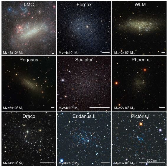Figure 1. Approaching the threshold of galaxy formation. Shown are images of dwarf galaxies spanning six orders of magnitude in stellar mass. In each panel, the dwarf’s stellar mass is listed in the lower-left corner and a scale bar corresponding to 200 pc is shown in the lower-right corner. The LMC, WLM, and Pegasus are dwarf irregular (dIrr) galaxies that have gas and ongoing star formation. The remaining six galaxies shown are gas-free dwarf spheroidal (dSph) galaxies and are not currently forming stars. The faintest galaxies shown here are only detectable in limited volumes around the Milky Way; future surveys may reveal many more such galaxies at greater distances. Image credits: Eckhard Slawik (LMC); ESO/Digitized Sky Survey 2 (Fornax); Massey et al. (2007; WLM, Pegasus, Phoenix); ESO (Sculptor); Mischa Schirmer (Draco), Vasily Belokurov and Sergey Koposov (Eridanus II, Pictoris I).

1.2. Overview of the ΛCDM model

The ΛCDM model of cosmology is the culmination of century of work on the physics of structure formation within the framework of general relativity. It also indicates the confluence of particle physics and astrophysics over the past four decades: the particle nature of dark matter directly determines essential properties of non-linear cosmological structure. While the ΛCDM model is phenomenological at present – the actual physics of dark matter and dark energy remain as major theoretical issues – it is highly successful at explaining the large-scale structure of the Universe and basic properties of galaxies that form within dark matter halos.

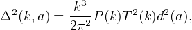
In the ΛCDM model, cosmic structure is seeded by primordial adiabatic fluctuations and grows by gravitational instability in an expanding background. The primordial power spectrum as a function of wavenumber k is nearly scale-invariant ¹, P(k) ∝ kⁿ with n ≃ 1. Scales that re-enter the horizon when the Universe is radiation-dominated grow extremely slowly until the epoch of matter domination, leaving a scale-dependent suppression of the primordial power spectrum that goes as k⁻⁴ at large k. This suppression of power is encapsulated by the “transfer function” T(k), which is defined as the ratio of amplitude of a density perturbation in the post-recombination era to its primordial value as a function of perturbation wavenumber k. This processed power spectrum is the input for structure formation calculations; the dimensionless processed power spectrum, defined by

(1)

therefore rises as k⁴ for scales larger than the comoving horizon at matter-radiation equality (corresponding to k = 0.008 Mpc⁻¹) and is approximately independent of k for scales that re-enter the horizon well before matter-radiation equality. Here, d(a) is the linear growth function, normalized to unity at a = 1. The processed z = 0 (a = 1) linear power spectrum for ΛCDM is shown by the solid line in Figure 2. The asymptotic shape behavior is most easily seen in the bottom panel, which spans the wave number range of cosmological interest. For a more complete discussion of primordial fluctuations and the processed power spectrum we recommend that readers consult Mo, van den Bosch & White (2010).

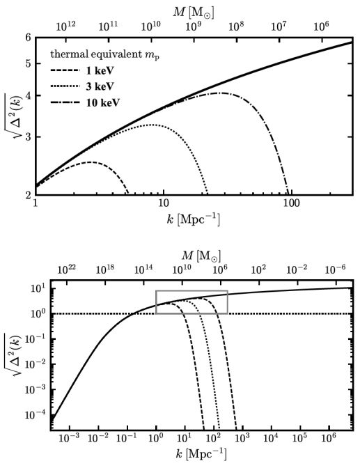Figure 2. The ΛCDM dimensionless power spectrum (solid lines, Equation 1) plotted as a function of linear wavenumber k (bottom axis) and corresponding linear mass Ml (top axis). The bottom panel spans all physical scales relevant for standard CDM models, from the particle horizon to the free-streaming scale for dark matter composed of standard 100 GeV WIMPs on the far right. The top panel zooms in on the scales of interest for this review, marked with a rectangle in the bottom panel. Known dwarf galaxies are consistent with occupying a relatively narrow 2 decade range of this parameter space – 109 − 1011 M⊙ – even though dwarf galaxies span approximately 7 decades in stellar mass. The effect of WDM models on the power spectrum is illustrated by the dashed, dotted, and dash-dotted lines, which map to the (thermal) WDM particle masses listed. See Section 3.2.1 for a discussion of power suppression in WDM.

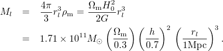
It is useful to associate each wavenumber with a mass scale set by its characteristic length r_l = λ / 2 = π / k. In the early Universe, when δ ≪ 1, the total amount of matter contained within a sphere of comoving Lagrangian radius r_l at z = 0 is

(2) (3)

The mapping between wave number and mass scale is illustrated by the top and bottom axis in Figure 2. The processed linear power spectrum for ΛCDM shown in the bottom panel (solid line) spans the horizon scale to a typical mass cutoff scale for the most common cold dark matter candidate (∼ 10⁻⁶ M_⊙; see discussion in Section 1.6). A line at Δ = 1 is plotted for reference, showing that fluctuations born on comoving length scales smaller than r_l ≈ 10 h⁻¹ Mpc ≈ 14 Mpc have gone non-linear today. The top panel is zoomed in on the small scales of relevance for this review (which we define more precisely below). Typical regions on these scales have collapsed into virialized objects today. These collapsed objects – dark matter halos – are the sites of galaxy formation.

1.3. Dark matter halos

1.3.1. Global properties. Soon after overdense regions of the Universe become non-linear, they stop expanding, turn around, and collapse, converting potential energy into kinetic energy in the process. The result is virialized dark matter halos with masses given by

(4)

where Δ ∼ 300 is the virial over-density parameter, defined here relative to the background matter density. As discussed below, the value of M_vir is ultimately a definition that requires some way of defining a halo's outer edge (R_vir). This is done via a choice for Δ. The numerical value for Δ is often chosen to match the over-density one predicts for a virialized dark matter region that has undergone an idealized spherical collapse (Bryan & Norman 1998), and we will follow that convention here. Note that given a virial mass M_vir, the virial radius, R_vir, is uniquely defined by Equation 4. Similarly, the virial velocity

(5)

is also uniquely defined. The parameters M_vir, R_vir, and V_vir are equivalent mass labels – any one determines the other two, given a specified over-density parameter Δ.

Galaxy Clusters: Mvir ≈ 1015 M⊙ Vvir ≈ 1000 km s−1

Milky Way Mvir ≈ 1012 M⊙ Vvir ≈ 100 km s−1

Smallest Dwarfs Mvir ≈ 109 M⊙ Vvir ≈ 10 km s−1

One nice implication of Equation 4 is that a present-day object with virial mass M_vir can be associated directly with a linear perturbation with mass M_l. Equating the two gives

(6)

We see that a collapsed halo of size R_vir is approximately 7 times smaller in physical dimension than the comoving linear scale associated with that mass today.

With this in mind, Equations 3-6 allow us to self-consistently define “small scales” for both the linear power spectrum and collapsed objects: M ≲ 10¹¹ M_⊙. As we will discuss, potential problems associated with galaxies inhabiting halos with V_vir ≃ 50 km s⁻¹ may point to a power spectrum that is non-CDM-like at scales r_l ≲ 1 Mpc.

WE DEFINE “SMALL SCALES” AS THOSE SMALLER THAN:

As alluded to above, a common point of confusion is that the halo mass definition is subject to the assumed value of Δ, which can vary by a factor of ∼ 3 depending on the author. For the spherical collapse definition, Δ ≃ 333 at z = 0 (for our fiducial cosmology) and asymptotes to Δ = 178 at high redshift (Bryan & Norman 1998). Another common choice is a fixed Δ = 200 at all z (often labeled M_200m in the literature). Finally, some authors prefer to define the virial overdensity as 200 times the critical density, which, according to Equation 4 would mean Δ(z) = 200 ρ_c(z)/ρ_m(z). Such a mass is commonly labeled “M₂₀₀” in the literature. For most purposes (e.g., counting halos), the precise choice does not matter, as long as one is consistent with the definition of halo mass throughout an analysis: every halo has the same center, but its outer radius (and mass contained within that radius) shifts depending on the definition. In what follows, we use the spherical collapse definition (Δ = 333 at z = 0) and adhere to the convention of labeling that mass “M_vir”.

Before moving on, we note that it is also possible (and perhaps even preferable) to give a halo a “mass” label that is directly tied to a physical feature associated with a collapsed dark matter object rather than simply adopting a Δ. More, Diemer & Kravtsov (2015) have advocated the use of a “splash-back” radius , where the density profile shows a sharp break (this typically occurs at ∼ 2 R_vir). Another common choice is to tag halos based not on a mass but on V_max, which is the peak value of the circular velocity V_c(r) = √G M(< r) / r as one steps out from the halo center. For any individual halo, the value of V_max (≳ V_vir) is linked to the internal mass profile or density profile of the system, which is the subject of the next subsection. As discussed below, the ratio V_max / V_vir increases as the halo mass decreases.

ROBUST PREDICTIONS FROM CDM-ONLY SIMULATIONS A defining characteristic of CDM-based hierarchical structure formation is that the smallest scales collapse first – a fact that arises directly from the shape of the power spectrum (Figure 1) and that lies at the heart of many robust predictions for the counts and structure of dark matter halos today. As discussed below, baryonic processes can alter these predictions to various degrees, but pure dark matter simulations have provided a well-defined set of basic predictions used to benchmark the theory.

The dark matter profiles of individual halos are cuspy and dense [Figure 3] The density profiles of individual ΛCDM halos increase steadily towards small radii, with an overall normalization and detailed shape that reflects the halo's mass assembly. At fixed mass, early-forming halos tend to be denser than later-forming halos. As with the mass function, both the shape and normalization of dark matter halo density structure is predicted by ΛCDM, with a well-quantified prediction for the scatter in halo concentration at fixed mass.

There are many more small halos than large ones [Figure 4] The comoving number density of dark matter halos rises steeply towards small masses, dn / dM ∝ Mα with α ≃ −1.9. At large halo masses, counts fall off exponentially above the mass scale that is just going non-linear today. Importantly, both the shape and normalization of the mass function is robustly predicted by the theory.

Substructure is abundant and almost self-similar [Figure 5] Dark matter halos are filled with substructure, with a mass function that rises as dN / dm ∝ mαs with αs ≃ −1.8 down to the low-mass free-streaming scale (m ≪ 1 M⊙ for canonical models). Substructure reflects the high-density cores of smaller merging halos that survive the hierarchical assembly process. Substructure counts are nearly self-similar with host mass, with the most massive subhalos seen at mmax ∼ 0.2 Mhost.

1.3.2. Abundance. In principle, the mapping between the initial spectrum of density fluctuations at z → ∞ and the mass spectrum of collapsed (virialized) dark matter halos at later times could be extremely complicated: as a given scale becomes non-linear, it could affect the collapse of nearby regions or larger scales. In practice, however, the mass spectrum of dark matter halos can be modeled remarkably well with a few simple assumptions. The first of these was taken by Press & Schechter (1974), who assumed that the mass spectrum of collapsed objects could be calculated by extrapolating the overdensity field using linear theory even into the highly non-linear regime and using a spherical collapse model (Gunn & Gott (1972)). In the Press-Schechter model, the dark matter halo mass function – the abundance of dark matter halos per unit mass per unit volume at redshift z, often written as n(M, z) – depends only on the rms amplitude of the linear dark matter power spectrum, smoothed using a spherical tophat filter in real space and extrapolated to redshift z using linear theory. Subsequent work has put this formalism on more rigorous mathematical footing (Bond et al. 1991, Cole 1991, Sheth, Mo & Tormen 2001), and this extended Press-Schechter (EPS) theory yields abundances of dark matter halos that are perhaps surprisingly accurate (see Zentner 2007 for a comprehensive review of EPS theory). This accuracy is tested through comparisons with large-scale numerical simulations.

Simulations and EPS theory both find a universal form for n(M, z): the comoving number density of dark matter halos is a power law with log slope of α ≃ −1.9 for M ≪ M^* and is exponentially suppressed for M ≫ M^*, where M^* = M^*(z) is the characteristic mass of fluctuations going non-linear at the redshift z of interest ². Importantly, given an initial power spectrum of density fluctuations, it is possible to make highly accurate predictions within ΛCDM for the abundance, clustering, and merger rates of dark matter halos at any cosmic epoch.

1.3.3. Internal structure. Dubinski & Carlberg (1991) were the first to use N-body simulations to show that the internal structure of a CDM dark matter halo does not follow a simple power-law, but rather bends from a steep outer profile to a mild inner cusp obeying ρ(r) ∼ 1 / r at small radii. More than twenty years later, simulations have progressed to the point that we now have a fairly robust understanding of the structure of ΛCDM halos and the important factors that govern halo-to-halo variance (e.g., Navarro et al. 2010, Diemer & Kravtsov 2015, Klypin et al. 2016), at least for dark-matter-only simulations.

To first approximation, dark matter halo profiles can be described by a nearly universal form over all masses, with a steep fall-off at large radii transitioning to mildly divergent cusp towards the center. A common way to characterize this is via the NFW functional form (Navarro, Frenk & White 1997), which provides a good (but not perfect) description dark matter profiles:

(7)

Here, r₋₂ is a characteristic radius where the log-slope of the density profile is −2, marking a transition point from the inner 1 / r cusp to an outer 1 / r³ profile. The second parameter, ρ₋₂, sets the value of ρ(r) at r = r₋₂. In practice, dark matter halos are better described the three-parameter Einasto (1965) profile (Navarro et al. 2004, Gao et al. 2008). However, for the small halos of most concern for this review, NFW fits do almost as well as Einasto in describing the density profiles of halos in simulations (Dutton & Macciò 2014). Given that the NFW form is slightly simpler, we have opted to adopt this approximation for illustrative purposes in this review.

As Equation 7 makes clear, two parameters (e.g., ρ₋₂ and r₋₂) are required to determine a halo's NFW density profile. For a fixed halo mass M_vir (which fixes R_vir), the second parameter is often expressed as the halo concentration: c = R_vir / r₋₂. Together, a M_vir − c combination completely specifies the profile. In the median, and over the mass and redshift regime of interest to this review, halo concentrations increase with decreasing mass and redshift: c ∝ M_vir^−a (1 + z)⁻¹, with a ≃ 0.1 (Bullock et al. 2001). Though halo concentration correlates with halo mass, there is significant scatter (∼ 0.1 dex) about the median at fixed M_vir (Jing 2000, Bullock et al. 2001). Some fraction of this scatter is driven by the variation in halo mass accretion history (Wechsler et al. 2002, Ludlow et al. 2016), with early-forming halos having higher concentrations at fixed final virial mass.

The dependence of halo profile on a mass-dependent concentration parameter and the correlation between formation time and concentration at fixed virial mass are caused by the hierarchical build-up of halos in ΛCDM: low-mass halos assemble earlier, when the mean density of the Universe is higher, and therefore have higher concentrations than high-mass halos (e.g., Navarro, Frenk & White 1997, Wechsler et al. 2002). At the very smallest masses, the concentration-mass relation likely flattens, reflecting the shape of the dimensionless power spectrum (see our Figure 1 and the discussion in Ludlow et al. 2016); at the highest masses and redshifts, characteristic of very rare peaks, the trend seems to reverse (a < 0; Klypin et al. 2016).

The right panel of Figure 3 summarizes the median NFW density profiles for z = 0 halos with masses that span those of large galaxy clusters (M_vir = 10¹⁵ M_⊙) to those of the smallest dwarf galaxies (M_vir = 10⁸ M_⊙). We assume the c − M_vir relation from Klypin et al. 2016. These profiles are plotted in physical units (unscaled to the virial radius) in order to emphasize that higher mass halos are denser at every radius than lower mass halos (at least in the median). However, at a fixed small fraction of the virial radius, small halos are slightly denser than larger ones. This is a result of the concentration-mass relation. Under the ansatz of abundance matching (Section 1.5, Figure 6), galaxy sizes (half-mass radii) track a fixed fraction of their host halo virial radius: r_gal ≃ 0.015 R_vir (Kravtsov 2013). This relation is plotted as a dotted line such that the dotted line intersects each solid line at that r = 0.015 R_vir, where R_vir is that particular halo’s virial radius. We see that small halos are slightly denser at the typical radii of the galaxies they host than are larger halos. Interestingly, however, the density range is remarkably small, with a local density of dark matter increasing by only a factor of ∼ 6 over the full mass range of halos that are expected to host galaxies, from the smallest dwarfs to the largest cD galaxies in the universe.

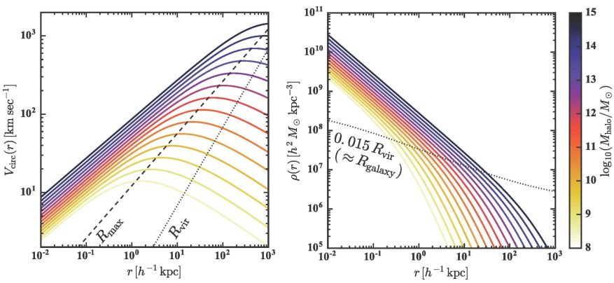Figure 3. Right: The density profiles of median NFW dark matter halos at z = 0 with masses that span galaxy clusters (Mvir = 1015 M⊙, black) to the approximate HI cooling threshold that is expected to correspond to the smallest dwarf galaxies (Mvir ≈ 108 M⊙, yellow). The lines are color coded by halo virial mass according to the bar on the right and are separated in mass by 0.5 dex. We see that (in the median) massive halos are denser than low-mass halos at a fixed physical radius. However, at a fixed small fraction of the virial radius, smaller halos are typically slightly denser than larger halos, reflecting the concentration-mass relation. This is demonstrated by the dotted line which connects ρ(r) evaluated at r = є Rvir for halos over a range of masses. We have chosen є = 0.015 because this value provides a good match to observed galaxy half-light radii over a wide range of galaxy luminosities under the assumption that galaxies occupy halos according to abundance matching (see Section 1.5 and Figure 6). Interestingly, the characteristic dark matter density at this ‘galaxy radius’ increases only by a factor of ∼ 6 over almost seven orders of magnitude in halo virial mass. Left: The equivalent circular velocity curves Vc(r) ≡ √G M(< r) / r for the same halos plotted on the right. The dashed line connects the radius Rmax where the circular velocity is maximum (Vmax) for each rotation curve. The dotted line tracks the Rvir – Vvir relation. The ratio Rmax / Rvir decreases towards smaller halos, reflecting the mass-concentration relation. The ratio Vmax / Vvir also increases with decreasing concentration.

1.4. Dark matter substructure

It was only just before the turn of the century that N-body simulations set within a cosmological CDM framework were able to robustly resolve the substructure within individual dark matter halos (Ghigna et al. 1998, Klypin et al. 1999a). It soon became clear that the dense centers of small halos are able to survive the hierarchical merging process: dark matter halos should be filled with substructure. Indeed, subhalo counts are nearly self-similar with host halo mass. This was seen as welcome news for cluster-mass halos, as the substructure could be easily identified with cluster galaxies. However, as we will discuss in the next section, the fact that Milky-Way-size halos are filled with substructure is less clearly consistent with what we see around the Galaxy.

Quantifying subhalo counts, however, is not so straightforward. Counting by mass is tricky because the definition of “mass” for an extended distribution orbiting within a collapsed halo is even more fraught with subjective decisions than virial mass. When a small halo is accreted into a large one, mass is preferentially stripped from the outside. Typically, the standard virial overdensity “edge” is subsumed by the ambient host halo. One option is to compute the mass that is bound to the subhalo, but even these masses vary from halo finder to halo finder. The value of a subhalo's V_max is better defined, and often serves as a good tag for quantifying halos.

Another option is to tag bound subhalos using the maximum virial mass that the halos had at the time they were first accreted ³ onto a host, M_peak. This is a useful option because stars in a central galaxy belonging to a halo at accretion will be more tightly bound than the dark matter. The resultant satellite's stellar mass is most certainly more closely related to M_peak than the bound dark matter mass that remains at z = 0. Moreover, the subsequent mass loss (and even V_max evolution) could change depending on the baryonic content of the host because of tidal heating and other dynamical effects (D'Onghia et al. 2010). For these reasons, we adopt M_sub = M_peak for illustrative purposes here.

The magenta lines in Figure 4 show the median subhalo mass functions (M_sub = M_peak) for four characteristic host halo masses (M_vir = 10¹²⁻¹⁴ M_⊙) according to the results of Rodríguez-Puebla et al. (2016). These lines are normalized to the right-hand vertical axis. Subhalos are counted only if they exist within the virial radius of the host, which means the counting volume increases as ∝ M_vir ∝ R_vir³ for these four lines. For comparison, the black line (normalized to the left vertical axis) shows the global halo mass function (as estimated via the fitting function from Sheth, Mo & Tormen 2001). The subhalo mass function rises with a similar (though slightly shallower) slope as the field halo mass function and is also roughly self-similar in host halo mass.

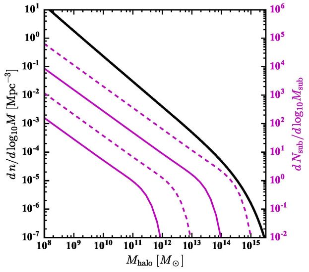Figure 4. Steep mass functions. The black solid line shows the z = 0 dark matter halo mass function (Mhalo = Mvir) for the full population of halos in the universe as approximated by Sheth, Mo & Tormen (2001). For comparison, the magenta lines show the subhalo mass functions at z = 0 (defined as Mhalo = Msub = Mpeak, see text) at the same redshift for host halos at four characteristic masses (Mvir = 1012, 1013, 1014, and 1015 M⊙) with units given along the right-hand axis. Note that the subhalo mass functions are almost self-similar with host mass, roughly shifting to the right by 10× for every decade increase in host mass. The low-mass slope of subhalo mass function is similar than the field halo mass function. Both field and subhalo mass functions are expected to rise steadily to the cutoff scale of the power spectrum, which for fiducial CDM scenarios is ≪ 1 M⊙.

1.5. Linking dark matter halos to galaxies

How do we associate dark matter halos with galaxies? One simple approximation is to assume that each halo is allotted its cosmic share of baryons f_b = Ω_b / Ω_m ≈ 0.15 and that those baryons are converted to stars with some constant efficiency є_⋆: M_⋆ = є_⋆ f_b M_vir. Unfortunately, as shown in Figure 5, this simple approximation fails miserably. Galaxy stellar masses do not scale linearly with halo mass; the relationship is much more complicated. Indeed, the goal of forward modeling galaxy formation from known physics within the ΛCDM framework is an entire field of its own (galaxy evolution; Somerville & Davé 2015). Though galaxy formation theory has progressed significantly in the last several decades, many problems remain unsolved.

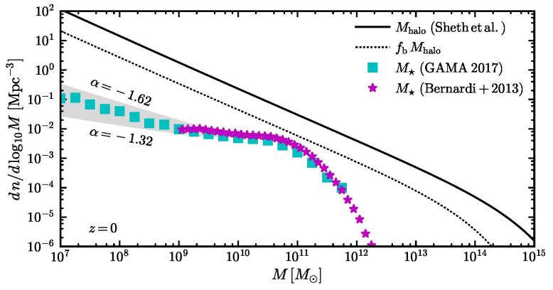Figure 5. The thick black line shows the global dark matter mass function. The dotted line is shifted to the left by the cosmic baryon fraction for each halo Mvir → fb Mvir. This is compared to the observed stellar mass function of galaxies from Bernardi et al. (2013, magenta stars) and Wright et al. (2017; cyan squares). The shaded bands demonstrate a range of faint-end slopes αg = −1.62 to −1.32. This range of power laws will produce dramatic differences at the scales of the classical Milky Way satellites (M⋆ ≃ 105−7 M⊙). Pushing large sky surveys down below 106 M⊙ in stellar mass, where the differences between the power law range shown would exceed a factor of ten, would provide a powerful constraint on our understanding of the low-mass behavior. Until then, this mass regime can only be explored with without large completeness corrections in vicinity of the Milky Way.

1.5.1. Abundance matching. As illustrated in Figure 5, the predicted mass function of collapsed dark matter halos has a considerably different normalization and shape than the observed stellar mass function of galaxies. The difference grows dramatically at both large and small masses, with a maximum efficiency of є_⋆≃ 0.2 at the stellar mass scale of the Milky Way (M_⋆ ≈ 10^10.75 M_⊙). This basic mismatch in shape has been understood since the earliest galaxy formation models set within the dark matter paradigm (White & Rees 1978) and is generally recognized as one of the primary constraints on feedback-regulated galaxy formation (White & Frenk 1991, Benson et al. 2003, Somerville & Davé 2015).

At the small masses that most concern this review, dark matter halo counts follow dn / dM ∝ M^α with a steep slope α_DM ≃ −1.9 compared to the observed stellar mass function slope of α_g = −1.47 (Baldry et al. 2012, which is consistent with the updated GAMA results shown in Figure 5). Current surveys that cover enough sky to provide a global field stellar mass function reach a completeness limit of M_⋆ ≈ 10^7.5 M_⊙. At this mass, galaxy counts are more than two orders of magnitude below the naive baryonic mass function f_b M_vir. The shaded band illustrates how the stellar mass function would extrapolate to the faint regime spanning a range of faint-end slopes α that are marginally consistent with observations at the completeness limit.

One clear implication of this comparison is that galaxy formation efficiency (є_⋆) must vary in a non-linear way as a function of M_vir (at least if ΛCDM is the correct underlying model). Perhaps the cleanest way to illustrate this is adopt the simple assumption of Abundance Matching (AM): that galaxies and dark matter halos are related in a one-to-one way, with the most massive galaxies inhabiting the most massive dark matter halos (Frenk et al. 1988, Kravtsov et al. 2004, Conroy, Wechsler & Kravtsov 2006, Moster et al. 2010, Behroozi, Wechsler & Conroy 2013). The results of such an exercise are presented in Figure 6 (as derived by Behroozi et al., in preparation). The gray band shows the median M_⋆ − M_vir relation with an assumed 0.2 dex of scatter in M_⋆ at fixed M_vir. The magenta band expands the scatter to 0.5 dex . This relation is truncated near the completeness limit in Baldry et al. (2012). The central dashed line in Figure 6 shows the median relation that comes from extrapolating the Baldry et al. (2012) mass function with their best-fit α_g = −1.47 down to the stellar mass regime of Local Group dwarfs. The cyan band brackets the range for the two other faint-end slopes shown in Figure 5: α_g = −1.62 and −1.32.

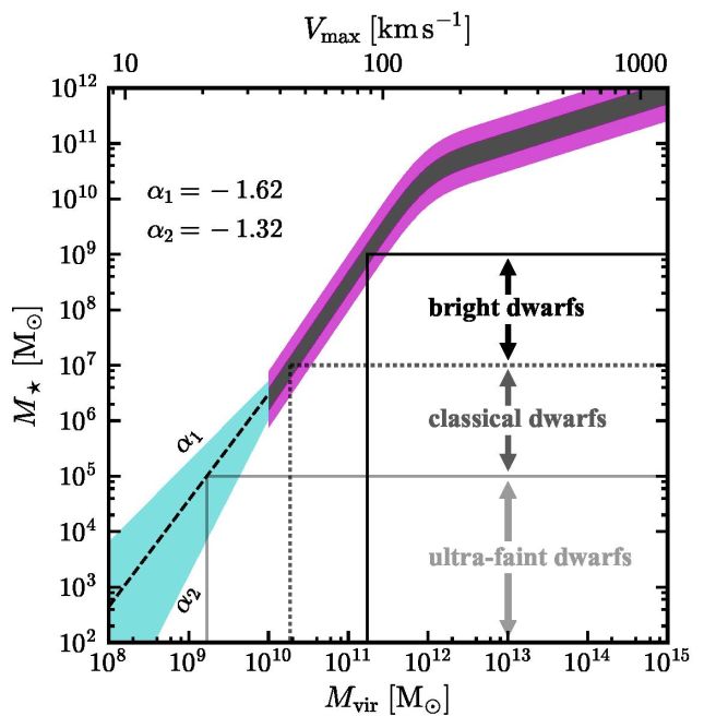Figure 6. Abundance matching relation from Behroozi et al. (in preparation). Gray (magenta) shows a scatter of 0.2 (0.5) dex about the median relation. The dashed line is power-law extrapolation below the regime where large sky surveys are currently complete. The cyan band shows how the extrapolation would change as the faint-end slope of the galaxy stellar mass function (α) is varied over the same range illustrated by the shaded gray band in Figure 5. Note that the enumeration of M⋆ = 105 M⊙ galaxies could provide a strong discriminator on faint-end slope, as the ± 0.15 range in α shown maps to an order of magnitude difference in the halo mass associated with this galaxy stellar mass and a corresponding factor of ∼ 10 shift in the galaxy/halo counts shown in Figure 4.

Figure 6 allows us to read off the virial mass expectations for galaxies of various sizes. We see that Bright Dwarfs at the limit of detection in large sky surveys (M_⋆ ≈ 10⁸ M_⊙) are naively associated with M_vir ≈ 10¹¹ M_⊙ halos. Galaxies with stellar masses similar to the Classical Dwarfs at M_⋆ ≈ 10⁶ M_⊙ are associated with M_vir ≈ 10¹⁰ M_⊙ halos. As we will discuss in Section 3, galaxies at this scale with M_⋆/M_vir ≈ 10⁻⁴ are at the critical scale where feedback from star formation may not be energetic enough to alter halo density profiles significantly. Finally, Ultra-faint Dwarfs with M_⋆ ≈ 10⁴ M_⊙, M_vir ≈ 10⁹ M_⊙, and M_⋆ / M_vir ≈ 10⁻⁵ likely sit at the low-mass extreme of galaxy formation.

Bright Dwarfs: M⋆ ≈ 108 M⊙ Mvir ≈ 1011M⊙ M⋆ / Mvir ≈ 10−3

Classical Dwarfs: M⋆ ≈ 106 M⊙ Mvir ≈ 1010 M⊙ M⋆ / Mvir ≈ 10−4

Ultra-faint Dwarfs: M⋆ ≈ 104 M⊙ Mvir ≈ 109 M⊙ M⋆ / Mvir ≈ 10−5

1.5.2. Kinematic Measures. An alternative way to connect to the dark matter halo hosting a galaxy is to determine the galaxy’s dark matter mass kinematically. This, of course, can only be done within a central radius probed by the baryons. For the small galaxies of concern for this review, extended mass measurements via weak lensing or hot gas emission is infeasible. Instead, masses (or mass profiles) must be inferred within some inner radius, defined either by the stellar extent of the system for dSphs and/or the outer rotation curves for rotationally-supported gas disks.

Bright dwarfs, especially those in the field, often have gas disks with ordered kinematics. If the gas extends far enough out, rotation curves can be extracted that extend as far as the flat part of the galaxy rotation curve V_flat. If care is taken to account for non-trivial velocity dispersions in the mass extraction (e.g., Kuzio de Naray, McGaugh & de Blok 2008), then we can associate V_flat ≈ V_max.

Owing to the difficulty in detecting them, the faintest galaxies known are all satellites of the Milky Way or M31 and are dSphs. These lack rotating gas components, so rotation curve measurements are impossible. Instead, dSphs are primarily stellar dispersion-supported systems, with masses that are best probed by velocity dispersion measurements obtained star-by-star for the closest dwarfs (e.g., Walker et al. 2009, Simon et al. 2011, Kirby et al. 2014). For systems of this kind, the mass can be measured accurately within the stellar half-light radius (Walker et al. 2009). The mass within the de-projected (3D) half-light radius (r_1/2) is relatively robust to uncertainties in the stellar velocity anisotropy and is given by M(< r_1/2) = 3 σ_⋆² r_1/2 / G, where σ_⋆ is the measured, luminosity-weighted line-of-sight velocity dispersion (Wolf et al. 2010). This formula is equivalent to saying that the circular velocity at the half-light radius is V_1/2 = V_c(r_1/2 ) = √3 σ_⋆. The value of V_1/2 (≤ V_max) provides a one-point measurement of the host halo's rotation curve at r = r_1/2.

1.6. Connections to particle physics

Although the idea of “dark” matter had been around since at least Zwicky (1933), it was not until rotation curve measurements of galaxies in the 1970s revealed the need for significant amounts of non-luminous matter (Freeman 1970, Rubin, Thonnard & Ford 1978, Bosma 1978, Rubin, Ford & Thonnard 1980) that dark matter was taken seriously by the broader astronomical community (and shortly thereafter, it was recognized that dwarf galaxies might serve as sensitive probes of dark matter; Aaronson 1983, Faber & Lin 1983, Lin & Faber 1983). Very quickly, particle physicists realized the potential implications for their discipline as well. Dark matter candidates were grouped into categories based on their effects on structure formation. “Hot” dark matter (HDM) particles remain relativistic until relatively late in the Universe’s evolution and smooth out perturbations even on super-galactic scales; “warm” dark matter (WDM) particles have smaller initial velocities, become non-relativistic earlier, and suppress perturbations on galactic scales (and smaller); and CDM has negligible thermal velocity and does not suppress structure formation on any scale relevant for galaxy formation. Standard Model neutrinos were initially an attractive (hot) dark matter candidate; by the mid-1980s, however, this possibility had been excluded on the basis of general phase-space arguments (Tremaine & Gunn 1979), the large-scale distribution of galaxies (White, Frenk & Davis 1983), and properties of dwarf galaxies (Lin & Faber 1983). The lack of a suitable Standard Model candidate for particle dark matter has led to significant work on particle physics extensions of the Standard Model. From a cosmology and galaxy formation perspective, the unknown particle nature of dark matter means that cosmologists must make assumptions about dark matters origins and particle physics properties and then investigate the resulting cosmological implications.

Cold Dark Matter (CDM) m ∼ 100 GeV, vthz=0 ≈ 0 km s−1

Warm Dark Matter (WDM) m ∼ 1 keV, vthz=0 ∼ 0.03 km s−1

Hot Dark Matter (HDM) m ∼ 1 eV, vthz=0 ∼ 30 km s−1

A general class of models that are appealing in their simplicity is that of thermal relics. Production and destruction of dark matter particles are in equilibrium so long as the temperature of the Universe kT is larger than the mass of the dark matter particle m_DM c². At lower temperatures, the abundance is exponentially suppressed, as destruction (via annihilation) dominates over production. At some point, the interaction rate of dark matter particles drops below the Hubble rate, however, and the dark matter particles “freeze out” at a fixed number density (see, e.g., Kolb & Turner 1994; this is also known as chemical decoupling). Amazingly, if the annihilation cross section is typical of weak-scale physics, the resulting freeze-out density of thermal relics with m ∼ 100 GeV is approximately equal to the observed density of dark matter today (e.g., Jungman, Kamionkowski & Griest 1996). This subset of thermal relics is referred to as weakly-interacting massive particles (WIMPs). The observation that new physics at the weak scale naturally leads to the correct abundance of dark matter in the form of WIMPs is known as the “WIMP miracle” (Feng & Kumar 2008) and has been the basic framework for dark matter over the past 30 years.

WIMPs are not the only viable dark matter candidate, however, and it is important to note that the WIMP miracle could be a red herring. Axions, which are particles invoked to explain the strong CP problem of quantum chromodynamics (QCD), and right-handed neutrinos (often called sterile neutrinos), which are a minimal extension to the Standard Model of particle physics that can explain the observed baryon asymmetry and why neutrino masses are so small compared to other fermions, are two other hypothetical particles that may be dark matter (among a veritable zoo of additional possibilities; see Feng 2010 for a recent review). While WIMPs, axions, and sterile neutrinos are capable of producing the observed abundance of dark matter in the present-day Universe, they can have very different effects on the mass spectrum of cosmological perturbations.

While the cosmological perturbation spectrum is initially set by physics in the very early universe (inflation in the standard scenario), the microphysics of dark matter affects the evolution of those fluctuations at later times. In the standard WIMP paradigm, the low-mass end of the CDM hierarchy is set by first collisional damping (subsequent to chemical decoupling but prior to kinetic decoupling of the WIMPs), followed by free-streaming (e.g., Hofmann, Schwarz & Stöcker 2001, Bertschinger 2006). For typical 100 GeV WIMP candidates, these processes erase cosmological perturbations with M ≲ 10⁻⁶ M_⊙ (i.e., Earth mass; Green, Hofmann & Schwarz 2004). Free-streaming also sets the low-mass end of the mass spectrum in models where sterile neutrinos decouple from the plasma while relativistic. In this case, the free-streaming scale can be approximated by the (comoving) size of the horizon when the sterile neutrinos become non-relativistic. The comoving horizon size at z = 10⁷, corresponding to m ≈ 2.5 keV, is approximately 50 kpc, which is significantly smaller than the scale derived above for L^* galaxies. keV-scale sterile neutrinos are therefore observationally-viable dark matter candidates (see Adhikari et al. 2016 for a recent, comprehensive review). QCD axions are typically ∼ µeV-scale particles but are produced out of thermal equilibrium (Kawasaki & Nakayama 2013). Their free-streaming scale is significantly smaller than that of a typical WIMP (see Section 3.2.1).

The previous paragraphs have focused on the effects of collisionless damping and free-streaming – direct consequences of the particle nature of dark matter – in the linear regime of structure formation. Dark matter microphysics can also affect the non-linear regime of structure formation. In particular, dark matter self-interactions – scattering between two dark matter particles – will affect the phase space distribution of dark matter. Within observational constraints, dark matter self-interactions could be relevant in the dense centers of dark matter halos. By transferring kinetic energy from high-velocity particles to low-velocity particles, scattering transfers “heat” to the centers of dark matter halos, reducing their central densities and making their velocity distributions nearly isothermal. This would have a direct effect on galaxy formation, as galaxies form within the centers of dark matter halos and the motions of their stars and gas trace the central gravitational potential. These effects are discussed further in Section 3.2.2.

The particle nature of dark matter is therefore reflected in the cosmological perturbation spectrum, in the abundance of collapsed dark matter structures as a function of mass, and in the density and velocity distribution of dark matter in virialized dark matter halos.

THREE CHALLENGES TO BASIC ΛCDM PREDICTIONS There are three classic problems associated with the small-scale predictions for dark matter in the ΛCDM framework. Other anomalies exist, including some that we discuss in this review, but these three are important because 1) they concern basic predictions about dark matter that are fundamental to the hierarchical nature of the theory; and 2) they have received significant attention in the literature.

Missing Satellites and Dwarfs [Figures 4-8] The observed stellar mass functions of field galaxies and satellite galaxies in the Local Group is much flatter at low masses than predicted dark matter halo mass functions: dn / dM⋆ ∝ M⋆αg with αg ≃ −1.5 (vs. α ≃ −1.9 for dark matter). The issue is most acute for Galactic satellites, where completeness issues are less of a concern. There are only ∼ 50 known galaxies with M⋆ > 300 M⊙ within 300 kpc of the Milky Way compared to as many as ∼ 1000 dark subhalos (with Msub > 107 M⊙) that could conceivably host galaxies. One solution to this problem is to posit that galaxy formation becomes increasingly inefficient as the halo mass drops. The smallest dark matter halos have simply failed to form stars altogether.

Low-density Cores vs. High-density Cusps [Figure 9] The central regions of dark-matter dominated galaxies as inferred from rotation curves tend to be both less dense (in normalization) and less cuspy (in inferred density profile slope) than predicted for standard ΛCDM halos (such as those plotted in Figure 3). An important question is whether baryonic feedback alters the structure of dark matter halos.

Too-Big-to-Fail [Figure 10] The local universe contains too few galaxies with central densities indicative of Mvir ≃ 1010 M⊙ halos. Halos of this mass are generally believed to be too massive to have failed to form stars, so the fact that they are missing is hard to understand. The stellar mass associated with this halo mass scale (M⋆≃ 106 M⊙, Figure 6) may be too small for baryonic processes to alter their halo structure (see Figure 13).

¹ Recent measurements find n = 0.968 ± 0.006 (Planck Collaboration et al. 2016), i.e., small but statistically different from true scale invariance. Back.

² The black line in Figure 4 illustrates the mass function of ΛCDM dark matter halos. Back.

³ This maximum mass is similar to the virial mass at the time of accretion, though infalling halos can begin losing mass prior to first crossing the virial radius. Back.