2. LOCAL MOMENTS: VARIANCES AND LINEAR REGRESSION

Let (x) be the field of mass-density fluctuations and g (x) the corresponding field of galaxy-density fluctuations, at a given time and for a given type of object. The fields are both smoothed with a fixed window which defines the term ``local''. The local biasing relation is considered to be a random process, specified by the biasing conditional distribution P(g | ). Let the one-point probability distribution functions (PDF) P() and P(g) be of zero means and standard deviations ² < ² > and _g² < g² >.

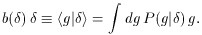
Define the mean biasing function b() by the conditional mean,

(1)

This function is plotted in Figure 1. It is a natural generalization of the deterministic linear biasing relation, g = b₁ . The function b() allows for any possible non-linear biasing. We find it useful to characterize the function b() by its moments and defined by

(2)

It will become clear that is the natural extension of b₁ and that / is the relevant measure of non-linearity, independent of stochasticity.

The local statistical character of the biasing can be expressed by the conditional moments of higher order about the mean at a given Define the random biasing field by g - < g | >, with < | > = 0. The local variance of at a given defines the biasing scatter function _b() and by averaging over one obtains the local biasing scatter parameter:

(3)

The scaling by ² is for convenience. The function < ² | >^1/2 is marked by error bars in Figure 1. Here and below we make use of a straightforward lemma, valid for any functions p(g) and q ():

(4)

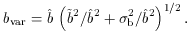
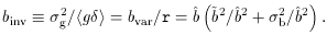
From the three basic parameters defined above one can derive other biasing parameters. A common one is the ratio of variances,

(5)

The second equality is a result of Eq. (4). It immediately shows that b_var is sensitive both to non-linearity and to stochasticity, with b_var . This makes b_var biased compared to ,

(6)

Using Eq. (4), the mean parameter is related to the covariance,

(7)

Thus, is the slope of the linear regression of g on , which makes it a natural generalization of b₁. Unlike the variance _g² in Eq. (5), the covariance in Eq. (7) has no contribution from _b. A complementary parameter to b_var is the linear correlation coefficient,

(8)

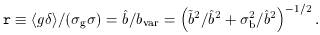
The ``inverse" regression, of on g, yields another biasing parameter:

(9)

Thus, b_inv is biased relative to , even more than b_var. The parameter b_inv is close to what is measured in practice by two-dimensional linear regression [52], because the errors in are larger than in g. Note that and _b nicely separate the non-linearity and stochasticity, while b_var, r and b_inv mix them.

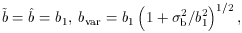
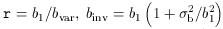
In the case of linear, stochastic biasing, the above parameters reduce to

(10)

Thus, b₁ b_var b_inv. In the case of non-linear deterministic biasing:

(11)

In the fully degenerate case of linear and deterministic biasing, all the b parameters are the same, and only then r = 1.

In actual applications, the above local biasing parameters are involved when the parameter ``'' is measured from observational data. For linear and deterministic biasing this parameter is defined unambiguously as ₁ f () / b₁, but any deviation from this model causes us to measure different 's by the different methods. For example, it is _var f () / b_var which is determined from _g and f (). The former is typically determined from a redshift survey, and the latter either from an analysis of peculiar velocity data, from the abundance of rich clusters, or by COBE normalization of a specific power-spectrum shape. In the case of stochastic biasing b_var is always an overestimate of , Eq. (5), and when the biasing is linear b_var is an overestimate of b₁. Therefore _var is underestimated accordingly.

Another useful way of estimate is via the linear regression of the fields in our cosmological neighborhood, e.g., - . v(x) on g (x) [17, 33, 52]. In the mildly-non-linear regime, - . v(x) is actually replaced by another function of the first spatial derivatives of the velocity field, which better approximates the scaled mass-density field f ()(x) [47]. The regression is effectively on g, because the errors in . v (or f ) are typically more than twice as large as the errors in g. Hence, the measured parameter is close to _inv f () / b_inv. In the case of linear and stochastic biasing, Eq. (10), b_inv is an overestimate of b₁ so the corresponding is underestimated accordingly.