


Direct constraints on the biasing field should be provided
by the data themselves, of galaxy density (e.g., from redshift surveys)
versus mass density (from peculiar velocity surveys, gravitational
lensing, etc.). A hint of scatter in the biasing relation
is the fact that the smoothed density peaks of the Great Attractor (GA)
and Perseus Pisces (PP) are of comparable height in the mass distribution
as recovered by POTENT from observed velocities
[15,
13,
19],
while PP is higher than GA in the galaxy maps
[33,
52].
Another piece of indirect evidence for scatter comes from
a linear regression of the 1200km s-1-smoothed density fields
of POTENT
mass and optical galaxies in our cosmological neighborhood, which
yields a
 2 ~ 2 per degree of
freedom [33].
One way to obtain a more reasonable
2 ~ 1
is to assume a biasing scatter of
2 ~ 2 per degree of
freedom [33].
One way to obtain a more reasonable
2 ~ 1
is to assume a biasing scatter of
 b ~ 0.5
(while ~ 0.3 at that smoothing).
With b1 ~ 1, one has
b2 /
b12 ~ 0.25.
This is only a crude estimate; there is yet much to be done with future data
along the lines of reconstructing the ``biasing field" in a given
region of space.
b ~ 0.5
(while ~ 0.3 at that smoothing).
With b1 ~ 1, one has
b2 /
b12 ~ 0.25.
This is only a crude estimate; there is yet much to be done with future data
along the lines of reconstructing the ``biasing field" in a given
region of space.
We have recently worked out a
promising way to recover the mean biasing function
b( ) and
its associated parameters
) and
its associated parameters  and
and
 from a measured PDF of
the galaxy distribution
[53].
This method is inspired by a ``de-biasing" technique by
Narayanan & Weinberg
[44].
If the biasing relation
g() were deterministic
and monotonic,
then it could be derived directly from the cumulative PDFs of
galaxies and mass, Cg(g) and
Cd(), via
from a measured PDF of
the galaxy distribution
[53].
This method is inspired by a ``de-biasing" technique by
Narayanan & Weinberg
[44].
If the biasing relation
g() were deterministic
and monotonic,
then it could be derived directly from the cumulative PDFs of
galaxies and mass, Cg(g) and
Cd(), via
We find, using halos in N-body simulations, that this is a good
approximation for <g|
Figure 2. The PDFs and the mean biasing
function, from a cosmological N-body
simulation of
The other key point is that the cumulative PDF of mass density is
relatively insensitive to the cosmological model or the power spectrum of
density fluctuations
[4,
5].
We find [53], using
a series of N-body simulations
of the CDM family of models in a flat or an open universe
with and without a tilt in the power spectrum,
that, compared to the differences between Cg and
C, the latter
can always be properly approximated by a cumulative log-normal distribution
of 1 +
 >
despite the significant scatter about it.
This is demonstrated in Figure 2.
>
despite the significant scatter about it.
This is demonstrated in Figure 2.
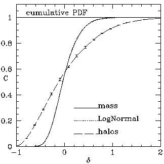
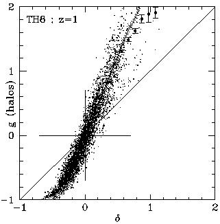
8 =
0.3 (z = 1)
with top-hat smoothing of 8 h Mpc and for halos of
M > 2 x 10¹²
M Left: the cumulative probability distributions C of density
fluctuations
of halos (g) and of mass ().
A log-normal distribution is shown for comparison.
The errors are by bootstrap re-sampling of halos.
The horizontal separation between the curves approximates the mean
biasing function <g|> =
b()2
at the corresponding value of .
Right: the density fields of halos and mass compared at grid points.
The symbols describe the mean biasing function as derived
from this data in bins.
The solid curve is derived from the PDFs via Eq. (21). The dotted
lines mark the error corresponding to the error in the PDF.
(Based on [53].)
with a single parameter
.
Deviations may show up in the extreme tails of the distribution
[5],
which may affect the skewness and higher moments but are of little
concern for our purpose here. This means that in order to evaluate
b()
one only needs to measure Cg(g) from a galaxy
density field,
and add the rms of mass
fluctuations at the same smoothing scale.
Since the redshift surveys are by far richer and more extended than
peculiar-velocity samples, this method will allow a much better handle
on b() than the local
comparison of density fields of galaxies and mass.
Left: the cumulative probability distributions C of density
fluctuations
of halos (g) and of mass ().
A log-normal distribution is shown for comparison.
The errors are by bootstrap re-sampling of halos.
The horizontal separation between the curves approximates the mean
biasing function <g|> =
b()2
at the corresponding value of .
Right: the density fields of halos and mass compared at grid points.
The symbols describe the mean biasing function as derived
from this data in bins.
The solid curve is derived from the PDFs via Eq. (21). The dotted
lines mark the error corresponding to the error in the PDF.
(Based on [53].)
with a single parameter
.
Deviations may show up in the extreme tails of the distribution
[5],
which may affect the skewness and higher moments but are of little
concern for our purpose here. This means that in order to evaluate
b()
one only needs to measure Cg(g) from a galaxy
density field,
and add the rms of mass
fluctuations at the same smoothing scale.
Since the redshift surveys are by far richer and more extended than
peculiar-velocity samples, this method will allow a much better handle
on b() than the local
comparison of density fields of galaxies and mass.