


Any measurement of a function of h,  m, and
  can be
included in a joint likelihood
can be
included in a joint likelihood
which I take as the product of seven of the most recent independent
cosmological constraints
(Table 1 and Fig. 3).
For example, one of the
Figure 3. The regions of the
(
Another
The (
This complementarity is even more important
(but more difficult to visualize) in three-dimensional parameter space:
(h,
This has the advantage of explicitly displaying the h dependence of
the t result.
The joint likelihood
Figure 4. This plot shows the region of the
h - t0 plane preferred by the combination of
all seven constraints.
The result, t0 = 13.4 ± 1.6 Ga, is the main
result of this paper.
The thick contours around the best fit (indicated by a star) are at
likelihood levels defined by
What one uses for
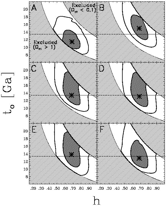
Figure 5. The purpose of this figure is to
show how Fig. 4 is built up from
the seven independent constraints used in the analysis.
All six panels are analogous to Fig. 4 but
contain only the Hubble constraint [h = 0.68 ± 0.10, (Eq. 2)]
convolved with a single constraint:
(A) cosmic microwave background, (B) SNe,
(C) cluster mass-to-light ratios, (D) cluster
abundance evolution,
(E) double radio lobes, and (F) baryons
(Table 1).
The relative position of the best fit (indicated by a star) and the
13.4-Ga line indicates
how each constraint contributes to the result.
To show how each constraint contributes to the result,
I convolved each constraint separately with Eq. 2
(Fig. 5).
The result does not depend strongly on any one of the constraints (see
``all - x'' results in Table 2).
For example, the age, independent of the SNe data, is
t0(all - SNe) =
13.3+1.7-1.8 Ga, which differs negligibly from
the main result. The age,
independent of the SNe and CMB data, is
Table 2: Age estimates of our
Galaxy and
universe (36).
``Technique'' refers to the method used to make the age estimate.
OC, open clusters; WD, white dwarfs; LF, luminosity function; GC,
globular clusters;
M/L, mass-to-light ratio; and cl evol, cluster abundance evolution.
The averages are inverse variance-weighted averages of the individual
measurements. The sun is not included in the disk average.
``Isotopes'' refers to the use of relative isotopic abundances of
long-lived species as indicated by absorption
lines in spectra of old disk stars.
The ``stellar ages'' technique uses main sequence fitting and the new
Hipparcos subdwarf calibration.
``All'' means that all six constraints in
Table 1 and the CMB
constraints were used in Eq. 1.
``All-x'' means that all seven constraints except constraint x were used
in Eq. 1.
Figures 3 and 5 and the
all - x results indicate a high level of agreement
between constraints and the lack of dependence on any single constraint.
Thus, there is a broad consistency between the ages preferred by the CMB
and the six other independent constraints.
Figure 2 presents all of the
disk and halo age estimates.
 i in Eq. 1 represents
the constraints on h.
Recent measurements can be summarized
as
i in Eq. 1 represents
the constraints on h.
Recent measurements can be summarized
as  = 0.68 ± 0.10
(16).
I represent these measurements in Eq. 1 by the likelihood,
= 0.68 ± 0.10
(16).
I represent these measurements in Eq. 1 by the likelihood,
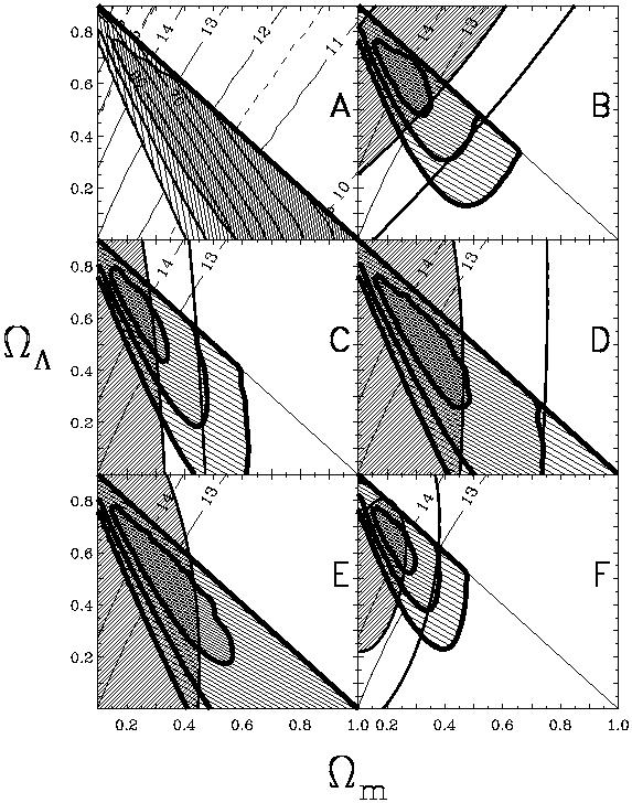
m,
)
plane preferred by various constraints.
(A) Cosmic microwave background, (B) SNe,
(C) cluster mass-to-light ratios, (D) cluster
abundance evolution,
(E) double radio lobes, and (F) all combined.
The power of combining CMB constraints with each of the other
constraints (Table 1) is also shown.
The elongated triangles (from upper left to lower right) in
(A) are the approximate
1 ,
2 and
3 confidence levels of the likelihood
from CMB data, CMB
(9).
(A) also shows the important h dependence of
CMB.
The contours within the dark shaded region are of h values that
maximize CMB for a given
(m,
) pair
(h = 0.70, 0.90 contours are labeled).
This correlation between preferred h and preferred
(m,
) helps
CMB(h,
m,
) constrain t0.
In (B) through (E), thin contours enclose the
1
(shaded) and 2 confidence regions
from separate constraints, and thick contours indicate the
1,
2 and
3 regions of the combination of
CMB with
these same constraints. (F) shows the region preferred by
the combination of the separate constraints shown in (B)
through (E) (thin contours) as well as the combination
of (A) through (E) (thick contours).
The best fit values are = 0.65 ± 0.13 and
m = 0.23 ± 0.08.
In (A), the thin iso-t0 contours (labeled
``10'' through ``14'') indicate the age in Ga
when h = 0.68 is assumed.
For reference, the 13- and 14-Ga contours are in all the panels.
To give an idea of the sensitivity of the h dependence of these
contours, the two additional dashed
contours in (A) show the 13-Ga contours for h = 0.58 and
h = 0.78 (the 1 limits of
the principle h estimate used in this paper).
In (F), it appears that the best fit has t0
,
2 and
3 confidence levels of the likelihood
from CMB data, CMB
(9).
(A) also shows the important h dependence of
CMB.
The contours within the dark shaded region are of h values that
maximize CMB for a given
(m,
) pair
(h = 0.70, 0.90 contours are labeled).
This correlation between preferred h and preferred
(m,
) helps
CMB(h,
m,
) constrain t0.
In (B) through (E), thin contours enclose the
1
(shaded) and 2 confidence regions
from separate constraints, and thick contours indicate the
1,
2 and
3 regions of the combination of
CMB with
these same constraints. (F) shows the region preferred by
the combination of the separate constraints shown in (B)
through (E) (thin contours) as well as the combination
of (A) through (E) (thick contours).
The best fit values are = 0.65 ± 0.13 and
m = 0.23 ± 0.08.
In (A), the thin iso-t0 contours (labeled
``10'' through ``14'') indicate the age in Ga
when h = 0.68 is assumed.
For reference, the 13- and 14-Ga contours are in all the panels.
To give an idea of the sensitivity of the h dependence of these
contours, the two additional dashed
contours in (A) show the 13-Ga contours for h = 0.58 and
h = 0.78 (the 1 limits of
the principle h estimate used in this paper).
In (F), it appears that the best fit has t0
 14.5 Ga, but
all constraints shown here are independent of information about h;
they do not include the h dependence of CMB, baryons
or Hubble
(Table 1).
14.5 Ga, but
all constraints shown here are independent of information about h;
they do not include the h dependence of CMB, baryons
or Hubble
(Table 1).
errors in the likelihood analysis.
The first four constraints are plotted in
Fig. 3 B through E.
Method Reference Estimate
SNe (35)
m=0 = -0.28 ± 0.16
mflat = 0.27 ± 0.14
Cluster mass-to-light
(6)
m=0 = 0.19 ± 0.14
Cluster abundance evolution
(7)
m=0 = 0.170.28-0.10
mflat =
0.22+0.25-0.10
Double radio sources
(8)
m=0 = -0.25+0.70-0.50
mflat =
0.1+0.50-0.20
Baryons
(19)
m h2/3 = 0.19 ± 0.12
Hubble
(16)
h = 0.68 ± 0.10
i
in Eq. 1 comes from measurements of
the fraction of normal baryonic matter in clusters of galaxies
(14)
and estimates of the density of normal baryonic matter in the universe
[bh2 = 0.015 ± 0.005
(15,
18)].
When combined, these measurements yield
 = 0.19 ± 0.12
(19),
which contributes to the likelihood through
= 0.19 ± 0.12
(19),
which contributes to the likelihood through
 m,
)-dependencies of the remaining five constraints are
plotted in Fig. 3
(20).
The 68% confidence level regions derived from CMB and SNe
(Fig. 3, A and B)
are nearly orthogonal, and the region of overlap is relatively small.
Similar complementarity exists between the
CMB and the other data sets
(Figs. 3, C through E).
The combination of them all (Fig. 3F) yields
= 0.65 ± 0.13 and m = 0.23 ± 0.08
(21).
m,
).
Although the CMB alone cannot tightly constrain any of these parameters,
it does have a strong preference in the three-dimensional space (h,
m,
). In Eq. 1, I used
CMB(h,
m,
), which is a generalization of
CMB(m, ) (Fig. 3A)
(22).
To convert the three-dimensional likelihood
(h,
m,
)
of Eq. 1 into an estimate of the
age of the universe and into a more easily
visualized two-dimensional likelihood,
(h,
t0), I computed the dynamic age
corresponding to each point in the three-dimensional space (h,
m,
).
For a given h and t0, I then set
(h,
t0) equal
to the maximum value of (h,
m,
)
m,
)-dependencies of the remaining five constraints are
plotted in Fig. 3
(20).
The 68% confidence level regions derived from CMB and SNe
(Fig. 3, A and B)
are nearly orthogonal, and the region of overlap is relatively small.
Similar complementarity exists between the
CMB and the other data sets
(Figs. 3, C through E).
The combination of them all (Fig. 3F) yields
= 0.65 ± 0.13 and m = 0.23 ± 0.08
(21).
m,
).
Although the CMB alone cannot tightly constrain any of these parameters,
it does have a strong preference in the three-dimensional space (h,
m,
). In Eq. 1, I used
CMB(h,
m,
), which is a generalization of
CMB(m, ) (Fig. 3A)
(22).
To convert the three-dimensional likelihood
(h,
m,
)
of Eq. 1 into an estimate of the
age of the universe and into a more easily
visualized two-dimensional likelihood,
(h,
t0), I computed the dynamic age
corresponding to each point in the three-dimensional space (h,
m,
).
For a given h and t0, I then set
(h,
t0) equal
to the maximum value of (h,
m,
)
 (h, t0) of Eq. 4
yields an age for the universe: t0 = 13.4 ± 1.6
Ga (Fig. 4).
This result is a billion years younger than
other recent age estimates.
(h, t0) of Eq. 4
yields an age for the universe: t0 = 13.4 ± 1.6
Ga (Fig. 4).
This result is a billion years younger than
other recent age estimates.

/ max = 0.607,
and 0.135,
which approximate 68% and 95% confidence levels, respectively.
These contours can be projected onto the t0 axis to
yield the age result.
This age result is robust to variations in the Hubble constraint
as indicated in Table 2.
The areas marked ``Excluded'' (here and in
Fig. 5) result from the
range of parameters considered:
0.1  m
1.0, 0
0.9 with m +
1.
Thus, the upper (high t0) boundary is defined by
(m,
) =
(0.1, 0.9), and the lower boundary
is the standard Einstein-deSitter model
defined by (m,
) = (1, 0). Both of these
boundary models are
plotted in Fig. 1.
The estimates from Table 2 of the age of our
Galactic halo (tGal) and the age of
the Milky Way (tdisk) are shaded grey. The universe is about
1 billion years older than our Galactic halo.
The combined constraints also yield a best fit value of the Hubble constant
which can be read off of the x axis (h = 0.73 ± 0.09, a
slightly higher and tighter estimate than the input h = 0.68
± 0.10).
Hubble(h) in Eq. 1 is particularly
important
because, in general, we expect the higher h values to yield
younger ages.
Table 2 contains results
from a variety of h estimates, assuming various central values
and various
uncertainties around these values.
The main result t = 13.4 ± 1.6 Ga has used h = 0.68 ±
0.10 but
does not depend strongly on the central value assumed for Hubble's constant
(as long as this central value is in the most accepted range, 0.64
h 0.72)
or on the uncertainty of h (unless this uncertainty is taken to be
very small).
Assuming an uncertainty of 0.10, age estimates from using h = 0.64,
0.68 and 0.72
are 13.5, 13.4 and 13.3 Ga, respectively
(Fig. 2).
Using a larger uncertainty of 0.15 with the same h values
does not substantially change the results, which are 13.4, 13.3, 13.2
Ga, respectively.
For both groups, the age difference is only 0.2 Gy.
If t0
m
1.0, 0
0.9 with m +
1.
Thus, the upper (high t0) boundary is defined by
(m,
) =
(0.1, 0.9), and the lower boundary
is the standard Einstein-deSitter model
defined by (m,
) = (1, 0). Both of these
boundary models are
plotted in Fig. 1.
The estimates from Table 2 of the age of our
Galactic halo (tGal) and the age of
the Milky Way (tdisk) are shaded grey. The universe is about
1 billion years older than our Galactic halo.
The combined constraints also yield a best fit value of the Hubble constant
which can be read off of the x axis (h = 0.73 ± 0.09, a
slightly higher and tighter estimate than the input h = 0.68
± 0.10).
Hubble(h) in Eq. 1 is particularly
important
because, in general, we expect the higher h values to yield
younger ages.
Table 2 contains results
from a variety of h estimates, assuming various central values
and various
uncertainties around these values.
The main result t = 13.4 ± 1.6 Ga has used h = 0.68 ±
0.10 but
does not depend strongly on the central value assumed for Hubble's constant
(as long as this central value is in the most accepted range, 0.64
h 0.72)
or on the uncertainty of h (unless this uncertainty is taken to be
very small).
Assuming an uncertainty of 0.10, age estimates from using h = 0.64,
0.68 and 0.72
are 13.5, 13.4 and 13.3 Ga, respectively
(Fig. 2).
Using a larger uncertainty of 0.15 with the same h values
does not substantially change the results, which are 13.4, 13.3, 13.2
Ga, respectively.
For both groups, the age difference is only 0.2 Gy.
If t0  1 /
h were adhered to, this age difference would be 1.6 Gy.
Outside the most accepted range the h dependence becomes stronger and
approaches
t0 1 /
h (23).
1 /
h were adhered to, this age difference would be 1.6 Gy.
Outside the most accepted range the h dependence becomes stronger and
approaches
t0 1 /
h (23).
Technique
Reference
h Assumptions
Age (Ga)
Object
Isotopes
(37)
None
4.53 ± 0.04
Sun
Stellar ages
(38)
None
8.0 ± 0.5
Disk OC
WD LF
(39)
None
8.0 ± 1.5
Disk WD
Stellar ages
(40)
None
9.0 ± 1
Disk OC
WD LF
(25)
None
9.7+0.9-0.8
Disk DW
Stellar ages
(41)
None
12.0+1.0-2.0
Disk OC
None
8.7 ± 0.4
tdisk(avg)
Stellar ages
(42)
None
11.5 ± 1.3
Halo GC
Stellar ages
(43)
None
11.8+1.1-1.3
Halo GC
Stellar ages
(44)
None
12 ± 1
Halo GC
Stellar ages
(45)
None
12 ± 1
Halo GC
Stellar ages
(46)
None
12.5 ± 1.5
Halo GC
Isotopes
(47)
None
13.0 ± 5
Halo stars
Stellar ages
(48)
None
13.5 ± 2
Halo GC
Stellar ages
(49)
None
14.0+2.3-1.6
Halo GC
None
12.2 ± 0.5
tGal (avg)
SNe
(4)
0.63 ± 0.0
14.5 ± 1.0
Universe
SNe (flat)
(4)
0.63 ± 0.0
14.9+1.4-1.1*
Universe
SNe
(5)
0.65 ± 0.02
14.2 ± 1.7
Universe
SNe (flat)
(5)
0.65 ± 0.02
15.2 ± 1.7*
Universe
All This work 0.60 ± 0.10
15.5+2.3-2.8
Universe
All This work 0.64 ± 0.10
13.5+3.5-2.2*
Universe
All This work 0.68 ± 0.10
13.4+1.6-1.6*
Universe
All This work 0.72 ± 0.10
13.3+1.2-1.9*
Universe
All This work 0.76 ± 0.10
12.3+1.9-1.6
Universe
All This work 0.80 ± 0.10
11.9+1.9-1.6
Universe
All This work 0.64 ± 0.02
14.6+1.6-1.1*
Universe
All - CMB This work 0.68 ± 0.10
14.0+3.0-2.2
Universe
All - SNe This work 0.68 ± 0.10
13.3+1.7-1.8
Universe
All - M/L This work 0.68 ± 0.10
13.3+1.9-1.7
Universe
All - cl evol This work 0.68 ± 0.10
13.3+1.7-1.4
Universe
All - radio This work 0.68 ± 0.10
13.3+1.7-1.5
Universe
All - baryons This work 0.68 ± 0.10
13.4+2.6-1.5
Universe
All - Hubble This work
None
< 14.2
Universe
All - CMB - SNe This work 0.68 ± 0.10
12.6+3.4-2.0
Universe
* Also plotted in Fig. 2.