


The new survey, which I undertook with my student John Spitzak, was made in a narrow "slice" at a declination of 23°, as illustrated by the gray region in Figure 6. The observations were made in a step-stare mode, keeping the telescope nearly pointing at the meridian while the sky rotated overhead. The region chosen is > 30° from the Galactic plane so that optical extinction is small. This region in Pisces-Perseus was chosen because Giovanelli & Haynes (1988) had so thoroughly observed the cataloged galaxies that "proposal pressure" at the Arecibo telescope in this time range was relatively low. In consequence we were able to obtain over 300 hours of telescope time, with which over 14,000 spectra were obtained, covering about 50 square degrees.
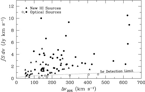
Because the region had been so thoroughly studied in HI before our survey, we have a direct test of our success rate. We rediscovered every previously-detected galaxy that we should have given our sensitivity limit. We illustrate this point in Figure 12. The sensitivity limit derived from this figure and from our more general arguments about signal and noise contributions for HI signals of various widths also permits us to determine more precisely what the limiting volume is for each of our detections. We use this information later when we derive an HI luminosity function.
|
Figure 12.
The integrated fluxes of sources detected in the Arecibo
slice survey. Detected sources are shown with solid symbols, while
undetected sources are shown with open symbols. A
5- |
In summary, the slice survey detected 79 objects within its redshift search range of 400-8400 km s-1. Half (38) of these were cataloged sources - found in one of the many optical catalogs contained in the NASA Extragalactic Database. The other half proved to be previously uncataloged objects, although almost all appear to have optical counterparts. This sample constitutes the largest collection of HI-selected objects yet found, and permits us to examine many of the questions raised in the earlier parts of this chapter.
The most fundamental question about these HI-selected objects is whether they represent a different population than the optically-selected sources or merely a deeper sample. For example, if optical and HI emission were exactly correlated, a deeper HI survey would pick up the same new sources as a deeper optical survey. If this were the case, the doubling in number of objects would imply an optical sample with a cutoff approximately 0.5 magnitude higher (i.e., a flux 21/3 times fainter). However, while the previously cataloged objects have a sharp cutoff fainter than a blue magnitude of about mB = 15.5, the new HI-selected sources have an average magnitude of mB = 17.5 (6.3 times fainter), with some objects beyond 20th magnitude (100 times fainter).
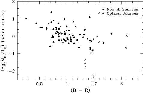
Another way of illustrating the sample differences is presented in Figure 13. First note that the newly-found, uncataloged objects (solid triangles) have significantly higher levels of HI relative to their optical output - up to ~ 10 × more solar masses of HI per solar luminosity of blue emission. The new objects also tend to be bluer than the previously cataloged optical sources, providing further evidence that these objects have different characteristics than an optically-selected sample. The blue colors of the new objects also demonstrate that the new objects should not have had any bias against their detection in optical surveys since most of these were conducted with photographic plates that are most sensitive in the blue.
|
Figure 13. Comparison of HI-to-optical luminosity ratio to the mean optical color of galaxies in the Arecibo slice survey. The colors are extinction corrected integrated values out to the 25 mag arcsec-2 isophote in the blue. |
It appears from Figure 13 that there is a trend in the characteristics of these galaxies: blue galaxies have a larger proportion of HI. I would speculate that this might be an indication that the new-found objects have undergone less star formation and that a larger proportion of their mass remains in a reservoir of HI.
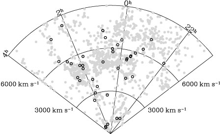
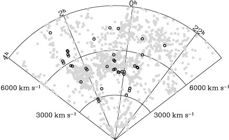
Another interesting question to examine is where these HI-selected sources lie relative to the large-scale structure defined by optically-selected sources. Dividing the sample into the cataloged and uncataloged parts, I illustrate the location of the objects in right ascension/redshift plots (often called slice diagrams) in Figures 15 and 14 respectively. For comparison, galaxies in the RC3 lying within ± 10° of the Arecibo slice (but excluding the slice area itself) are shown in gray. The large ridge of objects at ~ 5000 km s-1 is related to the Pisces-Perseus supercluster studied by Giovanelli & Haynes (1988).
|
Figure 14.
Locations of previously uncataloged galaxies found in the
Arecibo slice survey. The actual survey limits were from about 22h
to 3h, within the 23° <
|
|
Figure 15. Locations of previously cataloged galaxies "rediscovered" in the Arecibo slice survey, as in Figure 14. |
More uncataloged objects are found in the slice at low redshifts, but both the cataloged and uncataloged objects tend to follow the same large-scale structure seen throughout the region. This suggests that the voids are not populated by HI sources, but it must also be recognized that the sensitivity to low-mass HI sources only allows them to be detected to relatively small distances. In any case, it does not appear that HI sources will redraw the boundaries of large-scale structure, although it appears that the census of even the "Local Supercluster" (at redshifts below ~ 2000 km s-1) is incomplete.
 signal-to-noise line, based on equations 6 and
7, appears to successfully describe the boundary
of source detectability.
signal-to-noise line, based on equations 6 and
7, appears to successfully describe the boundary
of source detectability.
 < 24° declination band as
shown in
< 24° declination band as
shown in