2. Determination of Physical Parameters

In this section, we will concentrate on the impact of the physical input parameters on He abundance determinations. We will discuss the necessity of obtaining accurate line strengths and the limitations in doing so. We pay special attention to reddening as determined by H I line ratios. The uncertainties in this correction are particularly important as they feed into the uncertainty in all of the subsequent He I line strength determinations. We will also discuss determination of the electron temperature and density.

2.1. Measurements of Relative Emission Line Strengths and Errors

With the advent of large format, linear CCD array detectors in the last decade, we are in the best position ever to obtain spectra of emission line objects with the quality and accuracy necessary for helium abundance measurements. While it may seem unnecessary to discuss the measurement of emission line strengths here, this work starts with the assumption that the spectra have been properly calibrated and that errors associated with that calibration have been taken into account. Targets and standard stars should both be observed close to the parallactic angle in order to minimize atmospheric differential refraction (Filippenko 1982). It is important to observe several standard stars (preferably from the HST spectrophotometric standards of Oke 1990). These standard stars are believed to be reliable to about 1% across the optical spectrum, and thus, this sets a fundamental minimum level of uncertainty in any observed emission line ratio. Observations of both red and blue stars allows a check on the possibility of second-order contamination of the spectrum. Typically, one-dimensional spectra are extracted from long-slit (2-D) observations. Special care needs to be taken setting the extraction aperture width and the aperture should be sufficiently wide that small alignment errors do not give rise to systematic errors (this comes at a cost in signal/noise, but ensures photometric fidelity). Given these potential uncertainties, it is unreasonable to record errors of less than one percent in emission line ratios, regardless of the total number of photons recorded. Of course, multiple independent measurements of the same target provide the best estimates of true observational errors, and existing measurements of this type confirm this minimum error estimate (Skillman et al. 1994).

It should also be noted that it is imperative to integrate under the emission line profile (as opposed to fitting the line with a Gaussian profile). Fitting procedures can introduce systematic differences between high signal/noise and low signal/noise lines. Given the dynamic range of the H I and He I emission lines required to produce an accurate He/H abundance (e.g., the faint He I line 6678 is about 1% of H and He I 4026 is less than 2% of H), any systematic error between measuring strong and faint lines will have dramatic results. A special challenge is presented by the presence of underlying stellar absorption. The underlying absorption is generally broader than the emission, so quite often, when observed at a resolution of a few Angstroms or better, the H I or He I emission line is sitting in an absorption trough. Measuring all H I and He I emission lines in a consistent manner is important to obtaining a good solution for both the emission strength and the underlying absorption (see next section). Measurements at maximum resolution possible (while still measuring all lines simultaneously) are preferred.

2.2. Determination of Reddening and Underlying H I Absorption from Balmer Lines

Because (1) we know the theoretical emissivities of the recombination lines of H I (e.g., Hummer & Storey 1987), (2) the ratios of the H I recombination lines in emission are relatively insensitive to the physical conditions of the gas (i.e., electron temperature and density), and (3) there are a number of H I recombination lines spread through the optical spectrum, it is possible to use the observed line ratios to solve for the line-of-sight reddening of the spectrum (cf., Osterbrock 1989). If one assumes a reddening law (f(), e.g., Seaton 1979), in principle, it is possible to solve for the extinction as a function of wavelength by measuring a single pair of H I recombination lines. Values of C(H), the logarithmic reddening correction at H, can be derived from:

(1)

where I() is the intrinsic line intensity and F() is the observed line flux corrected for atmospheric extinction. Assuming a reddening law introduces a degree of uncertainty. Studies in our Galaxy have shown that the reddening law exhibits large variations between different lines of sight, but these variations are most important in the ultraviolet (Cardelli, Clayton, & Mathis 1989). Additionally, the total measured extinction can have both Galactic and extragalactic components (and note the added complexity of the shift in wavelength for the reddening law for systems at significant redshift). Note that it is typical that no error is associated with the assumption of a reddening law. Davidson & Kinman (1985) point out that tying the He I emission lines to the nearest pair of bracketing H I lines significantly reduces the impact of assuming a reddening law (i.e., "the interpolation advantage"), but it is unlikely that there is absolutely no error incurred with this assumption.

Underlying stellar absorption will affect the ratios of individual H I line pairs, so, in practice, it is best to measure several H I recombination lines. One can then solve for both the reddening and the stellar absorption underlying the emission lines (e.g., Shields & Searle 1978; Skillman 1985). It is generally assumed that the underlying absorption for the brightest Balmer H I lines is constant in terms of equivalent width. It is not clear how much error is incurred through this assumption, and inspection of stellar spectra shows that it is unlikely to be true for the fainter Balmer emission lines (e.g., H8, H9, and higher). However, one has the observational check of comparing these corrected lines to their theoretical values.

We recommend solving for the reddening and the underlying absorption by minimizing the differences between the observed and theoretical ratios for the three Balmer line ratios H / H, H / H, and H / H. Both H7 and H8 are blended with other emission lines, so they cannot be used for this purpose. While the H9 and H10 lines are often not observed with sufficient accuracy to constrain the reddening and absorption, in high quality spectra, the relative strengths of H9 and H10 provide a check on the derived solutions. In Appendix A we describe our method of using a ² minimization routine to determine the best values of C(H), the underlying equivalent width of hydrogen absorption (a_HI), and their associated errors.

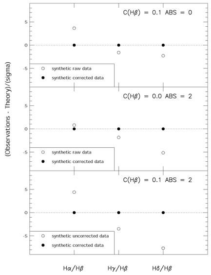
Figure 1 is presented for instructional purposes. It shows a comparison of the observed and corrected hydrogen Balmer emission line ratios for three synthetic cases. In constructing this figure, synthetic H I Balmer emission line spectra were calculated assuming an electron temperature (18,000 K), density (100 cm^-3), and H equivalent width (100 Å). Balmer emission line ratios were derived for three different combinations of reddening and absorption. All emission lines and equivalent widths were given uncertainties of 2%. In the first case, the spectrum was calculated assuming reddening and no underlying absorption. The second case assumes underlying absorption and no reddening. The third case has both. The open circles show the deviations of the original synthesized spectra from the theoretical ratios in terms of the synthesized uncertainties (2% for all lines). Note that reddening and underlying absorption induce corrections in the same direction for all three line ratios, i.e., the H / H line ratio increases for increased reddening and underlying absorption and the bluer Balmer line ratios all decrease for both effects. This covariance results in a degeneracy, thereby decreasing the diagnostic power of the corrections as we will show.

Figure 1. A comparison of the observed and corrected hydrogen Balmer emission line ratios for three synthetic cases (with no errors). The open circles show the deviations of the original synthesized spectra from the theoretical ratios in terms of the synthesized uncertainties (assumed to be 2% for all lines). The filled circles show the corrected values in the same manner. Note that the corrections for reddening and underlying absorption all have the same sense for all three line ratios, i.e., the H / H line ratio increases for increased reddening and underlying absorption and the higher order Balmer line ratios all decrease for both effects. This covariance results in decreased diagnostic power as shown in Figure 2.

The filled circles in Figure 1 show the results of using the ² minimization routine described in Appendix A. If such a minimization is used, then the ² should be reported. This allows one to make an independent check on the validity of the magnitude of the emission line uncertainties. As one can see, the minimization procedure accurately reproduces the assumed input parameters. In case 1, the minimization found C(H) = 0.10 ± 0.03 and a_HI = 0.00 ± 0.57. Similarly, for the other two cases, we find C(H) = 0.00 ± 0.03, a_HI = 2.00 ± 0.59 and C(H) = 0.10 ± 0.03, a_HI = 2.00 ± 0.59 respectively. In all three cases, since the data are synthetic, the ² values for the solutions are vanishingly small. Appendix B discusses cases from the literature where the ² values are quite large, indicating either a problem with the original spectrum, an underestimate of the emission line uncertainties, or both.

As a test to determine the appropriateness of the uncertainties for the values of C(H) and a_HI as produced by the ² minimization, we have run Monte Carlo simulations of the hydrogen Balmer ratios. The Monte Carlo procedure is described in Appendix A. Figure 2 shows the results of Monte Carlo simulations of solutions for the reddening and underlying absorption from hydrogen Balmer emission line ratios for three synthetic cases based on the input parameters of case 3 of Figure 1. That is, the original input spectra had reddening with C(H) = 0.1 and a_HI = 2 Å. For these values of C(H) and a_HI, we have run the Monte Carlo for three choices of EW(H) = 50, 100, and 200 Å. (EW(H) = 100 was used in Figure 1). Let us first concentrate on the results shown in the bottom panel of Figure 2. Each small point is the minimization solution derived from a different realization of the same input spectrum (with 2% errors in both emission line flux and equivalent width). The large open point with error bars shows the mean result with 1 errors derived from the ² solution from the original synthetic spectrum. The large filled point with error bars shows the mean result with 1 errors derived from the dispersion in the Monte Carlo solutions. Note that the covariance of the two parameters leads to error ellipses. The Monte Carlo simulations find the correct solutions, but the error bars appropriate to these solutions are significantly larger than the errors inferred from the single ² minimization. In this case there is a small offset in the mean solutions (mostly due to the fact that solutions with negative values are not allowed). In the bottom panel, the errors in C(H) are 29% larger and the errors in a_HI are about 61% larger for the Monte Carlo simulations compared to the single ² minimization.

Figure 2. The results of Monte Carlo simulations of solutions for the reddening and underlying absorption from hydrogen Balmer emission line ratios for three synthetic cases. Each small point is the solution derived from a different realization of the same input spectrum (with 2% errors in both emission line flux and equivalent width). The original input spectra had reddening with C(H) = 0.1 and aHI = 2 Å. The large filled point with error bars shows the mean result with 1 errors derived from the dispersion in the solutions. Note that the covariance of the two parameters leads to error ellipses. The Monte Carlo simulations find the correct solutions, but the error bars appropriate to these solutions are about twice the size of the errors inferred from single 2 minimizations. Note that the covariance of the two parameters leads to error ellipses. Note also that, given the input assumptions, that the constraints on the underlying absorption are stronger in absolute terms for the lower emission line equivalent width cases.

The middle and top panels of Figure 2 show cases for decreasing emission line equivalent width. Note that, given the input assumptions, the constraints on the underlying absorption are stronger in absolute terms for the lower emission line equivalent width cases. In all three cases, the ² minimization errors are smaller than those produced by the Monte Carlo simulations. For the middle panel, the differences are 41% for C(H) and 80% for a_HI, while for the top panel, the differences are 46% for C(H) and 86% for a_HI.

These test cases have shown that the errors in C(H) and the underlying stellar absorption can be underestimated by simply using the output from a ² minimization routine, and that Monte Carlo simulations can be used to give a more realistic estimate of the errors. Based on this experience, we recommend that the best way to determine the true uncertainties in the derived values of C(H) and a_HI is to run Monte Carlo simulations of the hydrogen Balmer ratios. Simply running a ² minimization will underestimate the uncertainty (due, in large part, to the covariance of the two parameters being solved for). Since the reddening correction must be applied to the He I lines as well, this uncertainty will propagate into the final estimation of the He abundance. This uncertainty, we find, is too large to be ignored.

If He I lines are observed at a given wavelength , their intensities relative to H after the reddening correction is given by eq. (1). The ratios I() / I(H) can then be used self-consistently to determine the He abundance and the physical parameters describing the HII regions, after the effects of collisional excitation, florescence, and underlying absorption as described in the next section. We can quantify the contribution to the overall He abundance uncertainty due to the reddening correction by propagating the error in eq. (1). Ignoring all other uncertainties in X_R() = I() / I(H), we would write

(2)

In the examples discussed above, _C(H) ~ 0.04 (from the Monte Carlo), and values of f are 0.237, 0.208, 0.109, -0.225, -0.345, -0.396, for He lines at 3889, 4026, 4471, 5876, 6678, 7065, respectively. For the bluer lines, this correction alone is 1 - 2% and must be added in quadrature to any other observational errors in X_R. For the redder lines, this uncertainty is 3 - 4%. This represents the minimum uncertainty which must be included in the individual He I emission line strengths relative to H. Note that these errors alone equal or exceed the 2% errors in the individual line strengths assumed for this exercise. However, the magnitude of the reddening error terms for the red lines can be reduced if these lines are compared directly to H. If the corrected H / H ratio is identical to the theoretical ratio, then it would be allowable to include only the uncertainty in the reddening difference between H and the red He I emission line. On the other hand, it is frequently the case that the corrected H / H ratio is significantly different from the theoretical ratio.

Finally, we should note that an additional complication is the possibility that, in the highest temperature (lowest metallicity) nebulae, the H line may be collisionally enhanced (Davidson & Kinman 1985; Skillman & Kennicutt 1993). In their detailed modeling of I Zw 18, Stasinska & Schaerer (1999) have found this to be an important effect (of order 7% enhancement in H). If this is not accounted for, this has the effect of artificially increasing the determined reddening (and thus, artificially decreasing the helium abundances measured from the lines redward of H (e.g., 5876, 6678) and increasing the helium abundances measured from lines blueward of H (e.g., 4471). More work along the lines Stasinska & Schaerer (1999) with photoionization modeling of high temperature nebulae is needed to determine whether this effect is common in these low metallicity regions.

2.3. Electron Temperature Determinations from Collisionally Excited Lines

Since the temperature is governed by the balance between the heating and cooling processes, and since the cooling is governed by different ionic species in different radial zones, one expects different ions to have different mean temperatures (cf. Stasinska 1990; Garnett 1992). While this is best treated with a complete photoionization model, a reasonable compromise is to treat the spectrum as if it arose in two different temperature zones, roughly corresponding to the O⁺ and O^{+ +} zones. Since the oxygen ions play a dominant role in the cooling, this is a reasonable thing to do. Deriving temperatures in the high ionization zone generally consists of measuring the highly temperature sensitive ratio of the emission from the "auroral line" of [O III] (4363) relative to the emission from the "nebular lines" of [O III] (4959,5007). Temperatures for the low ionization zone are usually derived from photoionization modeling (e.g., PSTE); although it is possible to derive temperatures in the low ionization zone from the [O II] I(7320 + 7330) / I(3726 + 3729) ratio and a similar ratio for [S II] (e.g., González-Delgado et al. 1994; PPR).

Note that, to date, usually only the temperature from the high ionization zone is used to derive the He abundance, and the He which resides in the low ionization zone is generally not dealt with in a self-consistent manner. To estimate the potential size of this effect, we can look at the data for SBS1159+545 from IT98. In SBS1159+545, 19% of the oxygen is in the O⁺ state (and thus 81% in the O^{+ +} state). Assuming all of the gas to be at a temperature of 18,400 K (the [O III] temperature), a 5876 / H ratio of 0.101 ± 0.002 yields a helium abundance of 0.0855 (before reduction to account for collisional enhancement and in agreement with IT98). Assuming 81% of the gas to be at the [O III] temperature of 18,400 K and 19% of the gas to be at the [O II] temperature of 15,200 K results in a helium abundance of 0.0848, or a difference of 0.8%. While this is a small difference, it is not negligible when compared to the reported uncertainty in the measurement. Curiously, including the effects of collisional enhancement almost perfectly cancels this effect for the reported density of 110 cm^-3 (y⁺ = 0.0815 treated as a single temperature zone and y⁺ = 0.0811 treated as two temperature zones for this object). Thus, using a lower temperature for the y⁺ in the O⁺ zone can increase or decrease the helium abundance depending on the density. The main point here is that the temperatures used for the two zones and the helium abundance should be treated consistently (as emphasized by PPR).

Steigman, Viegas, & Gruenwald (1997) have investigated the effect of internal temperature fluctuations on the derived helium abundances and find this to be important in the high temperature regime. The presence of temperature fluctuations, when analyzed assuming no temperature fluctuations, results in underestimating both the oxygen and helium abundances (here only [S II] densities are used, which are typically higher than the densities derived from He I lines). Assuming a range of relatively large temperature fluctuations (with a maximum of 4000K) results in an overall shift in the derived primordial helium abundance of about 3%. Steigman et al. have argued that, in absence of constraints on the temperature fluctuations, the errors should be increased to account for this uncertainty.

Peimbert, Peimbert, & Ruiz (2000) have shown that the different temperature dependences of the He I emission lines can be used to solve for the density, temperature, and helium abundance simultaneously and self-consistently. They point out that photoionization modeling consistently shows that the electron temperature derived from the [O III] lines is always an upper limit to the average temperature for the He I emission, and thus, assuming the [O III] temperature will always produce an upper limit to the true helium abundance. Here we will not explore the possibility of adding the electron temperature as a free parameter to our minimization routines. This is, in part, because the main motivations are to explore the method promoted by IT98, to explore the possibility of handling the effects of underlying absorption, and also, because one of our main conclusions, that Monte Carlo modeling is required for a true estimation of the errors will be true regardless of the minimization parameters. Nonetheless, this is a very important result with the implication that most helium abundances reported in the literature to date are really upper limits.

2.4. Electron Density Determinations from Collisionally Excited Lines

The average density can be derived by measuring the relative intensities of two collisionally excited lines which arise from a split upper level. In the "low density regime" collisional de-excitation is unimportant and all excitations are followed by emission of a photon. The ratio of the fluxes then simply reflects the ratio of the statistical weights of the two levels. In the "high density regime", where the level populations are held at the ratio of their statistical weights, the emission ratio becomes the ratio of the product of the statistical weights and the radiation transition probabilities. In the intermediate regime, near the "critical density" the line ratios are excellent density diagnostics. The best known is that of [S II] 6717 / 6731 which is sensitive in the range from 10² to 10⁴ cm^-3 and can be observed at moderate spectral resolution. At higher spectral resolution, one can use several other line pairs (e.g., [O II] 3726 / 3729).

In order to convert these line ratios into densities, one needs to know the energy level separations, the statistical weights of the levels, and the radiative and collisional excitation and de-excitation rates. Fortunately, one can use the five-level atom program originally written by De Robertis, Dufour, & Hunt (1987) which has been made generally available within IRAF ⁽¹⁾ by Shaw & Dufour (1995). This program has the additional great advantage that the authors have promised to keep the input atomic data updated.

As emphasized by ITL94, ITL97 and IT98, the [S II] line ratio suffers from two problems as a density diagnostic: (1) it is measuring the density is the low ionization zone, which may apply to less than 10% of the emission in a low metallicity giant HII region, and (2) it is relatively insensitive to density below about 100 cm^-3. Since the collisional excitation of the He I lines is important at the 1% level down to densities as low as 10 cm^-3, the [S II] lines are not ideal density indicators (cf. Izotov et al. 1999), and deriving densities directly from the He I lines is, in principle, preferable. This is discussed further in §4. However, calculating the density from the [S II] lines (and other collisionally excited lines) provides an excellent consistency check on the density derived from the He I lines.

¹ IRAF is distributed by the National Optical Astronomy Observatories, which is operated by the Association of Universities for Research in Astronomy, Inc. (AURA) under cooperative agreement with the National Science Foundation. Back.