4.5. Results

The outcome of applying VELMOD to the A82 + MAT subsample described above is presented in Figure 5. The VELMOD likelihood curves are shown both with and without the external quadrupole included. The formal likelihood is vastly improved when the quadrupole is included in the fit: since the likelihood statistic _forw is defined as -2ln[P(data| )], the ~ 20 point reduction in the minimum of _forw, minus the 5 extra degrees of freedom when the quadrupole is modeled, corresponds to a probability increase of a factor ~ e^7.5 2000. The improvement in formal likelihood through the addition of the quadrupole is so pronounced that we take the maximum likelihood value of _I from that fit, 0.492 ± 0.068, as our best estimate. However, the maximum likelihood estimate of _I when the quadrupole is neglected, 0.563 ± 0.074, differs from our best value at only the 1 level. While the quadrupole is important, it does not affect qualitatively our conclusions about the likely value of _I.

Figure 5. VELMOD likelihood statistic, forw (eq. [13]), plotted as a function of I for the real data. In the left-hand plot, an external quadrupole is modeled, as described in the text. In the right-hand plot, no external quadrupole is included in the velocity field. Cubic fits to the likelihood points are shown as dotted lines. The minima of the fitted curves, min, are the maximum likelihood estimates of I in each case. Note the very different values of the vertical axes of the two plots; this indicates the large increase in formal likelihood when the quadrupole is included.

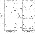
We can make several additional tests of the robustness of our results. Figure 6 shows how the likelihoods per object break down for fits to different cuts on the sample (see also Table 2). The left-hand panel plots _forw / N versus _I for the A82 and MAT samples separately, where N = 300 for A82 and N = 538 for MAT. Cubic fits to the individual sample likelihoods yield _I = 0.489 ± 0.084 and 0.498 ± 0.107 for A82 and MAT, respectively. This agreement is remarkable, given that there are only 53 galaxies in common between the two samples. Note that the -uncertainty is larger for the MAT sample, even though it contains nearly twice as many objects as the A82 sample. This is because the MAT objects typically lie at larger distances than do A82 objects, a property of the likelihood fit we now illustrate.

Figure 6. Breakdown of the VELMOD likelihood statistic among subsamples. The left-hand panel plots likelihood per point vs. I for the A82 and MAT samples individually. The right-hand panel plots likelihood per point vs. I for three different redshift intervals containing roughly the same number of objects. In each case, the minimum occurs within ~ 0.1 in I of the global minimum in forw at I = 0.492.

The right-hand panel of Figure 6 plots _forw / N versus _I for three subsamples in different redshift ranges. As Table 2 shows, the agreement in the derived values of _I is quite good. Changing the specific redshift intervals used for this test does not change the results significantly. Note that the -resolution decreases as one goes to higher redshift, despite the fact that there are nearly equal numbers of objects in each of the three redshift bins. This is because the likelihood is sensitive mainly to the fractional distance error in the IRAS prediction. Hence, nearby galaxies are more diagnostic of incorrect peculiar velocity predictions and thus of _I.

The fact that _forw / N decreases with redshift should not be interpreted as meaning that more distant objects are better fit by the velocity model. Instead, this decrease reflects a property of the VELMOD likelihood implicit in equation (15), which shows that the expectation value of _forw / N is ~ 1+ln (2) + ln[_TF² + (2.17 _v / [w(1 + u'(w))])²], which increases with decreasing cz in general. This effect will be particularly pronounced in flat zones (u' ~ -1) in the redshift-distance relation that are found in the Local Supercluster, which is why there is a marked difference between _forw / N for the A82 and MAT samples (the former preferentially populates the Local Supercluster region).

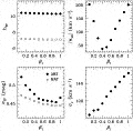
In Figure 7, we plot for the real data the same quantities plotted for a mock catalog in Figure 3, as well as the TF slopes. The slopes are extremely insensitive to _I. This indicates that the IRAS assigns low and high line width galaxies nearly the same relative distances at all _I. Significantly, the amplitude of the fitted Local Group velocity vector is minimized near the maximum likelihood value of _I, just as we saw with the mock catalog. This indicates once again that the fit attempts to compensate for a poor velocity field at very low and high _I by moving the Local Group. The mock catalogs showed us that the errors on the Cartesian components of w_LG are of order 50 km s^-1 (Table 1). Thus, the small value of w_LG obtained from VELMOD indicates that the Yahil et al. (1977) transformation to the Local Group barycenter is correct to within ~ 50 km s^-1, and that the Local Group has random velocity 50 km s^-1 relative to the mean peculiar velocity field in its neighborhood.

Figure 7. Left-hand panels: the TF slopes (top) and scatters (bottom), for the A82 and MAT samples, derived from VELMOD as a function of I. Right-hand panels: the amplitude of the Local Group random velocity vector (top) and the velocity noise v (bottom) derived from VELMOD as a function of I. All plots correspond to the run in which the quadrupole was modeled.

The lower right-hand panel of Figure 7 shows that _v increases monotonically with _I. Its maximum likelihood value is 125 km s^-1. This is a remarkably small number, when one considers that it includes not only the effect of random velocity noise but also of IRAS prediction error. In particular, if our estimate of the IRAS prediction error derived from our mock catalog experiments (Section 3.2), ~ 84 km s^-1, is roughly correct, our value for _v implies that the true one-dimensional velocity noise is 100 km s^-1. This result is consistent with past observations that the velocity field outside of clusters is "cold" (cf. Sandage 1986; Brown & Peebles 1987; Burstein 1990; Groth, Juszkiewicz, & Ostriker 1989; Strauss, Cen, & Ostriker 1993; Strauss, Ostriker, & Cen 1997). Finally, the lower left-hand panel demonstrates again what was seen earlier with the mock catalogs (Fig. 3), namely, that maximizing probability does not correspond to minimizing TF scatter. In large measure, this is because there is a trade-off between the variance due to the velocity noise _v and that due to the TF scatter. As _I approaches 1, _v gets steadily larger; _TF gets correspondingly smaller, despite the fact that the high-_I models are worse fits to the TF data. The TF scatters level out or rise only at _I 1.

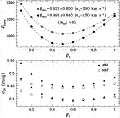
A final test of robustness involves eliminating the freedom in the VELMOD fit provided by the parameters w_LG and _v. One could argue that these parameters are like the quadrupole: they "are what they are," and we should not allow them to absorb the fit inaccuracies at the wrong value of _I. To assess this, we carried out two VELMOD runs in which w_LG was assumed to vanish identically. In the first run, we fixed the value of _v at 150 km s^-1, and in the second at 250 km s^-1. The quadrupole was held fixed at its best-fit value; the free parameters in this fit were limited to _I and the three TF parameters for each of the two samples. The results of this exercise are shown in Figure 8 and in Table 2. The derived values of _I differ inconsequentially from our best estimate obtained from the full fit. This shows that allowing ourselves the freedom to fit both w_LG and _v does not materially affect the derived value of _I. The formal uncertainties in _I are much reduced relative to the full fit because formerly free parameters have been held fixed. For _v = 150 km s^-1, the formal likelihood is worse than for the full fit, but only at the ~ 2 level. This reflects the fact that _v = 150 km s^-1 and w_LG = 0 themselves differ by only ~ 1 from their maximum likelihood values, according to our error estimates from Section 3.2. However, the formal likelihood for the _v = 250 km s^-1 run is considerably worse (by a factor of ~ 10^-7) than for the full fit. This shows that we rule out such a large _v at high significance.

Figure 8. Top panel: The VELMOD likelihood statistic forw as a function of I for a two runs in which the Local Group velocity vector was forced to vanish, and the velocity noise parameter v was held fixed at 150 and 250 km s-1. Although the formal likelihoods of the fit are worse than that of the full fit (cf. Fig. 5), particularly for v = 250 km s-1, the maximum likelihood estimates of I are nearly unchanged. Bottom panel: variation in the TF scatters TF, for the A82 and MAT samples, as a function of I for these VELMOD runs. The larger values correspond to the v = 150 km s-1 run. Note that the minimum derived TF scatters do not necessarily correspond to maximum likelihood (see text for further details).

The bottom panel of Figure 8 shows the fitted values of _TF as a function of _I for each of the two values of _v and for each of the two TF samples. The TF scatters now track the likelihood much better than they did in the full fit (bottom panel of Fig. 7); with _v fixed, maximizing likelihood is more nearly equivalent to minimizing TF scatter. However, they are still not the same thing: likelihood maximization occurs for _I 0.5, whereas TF scatter is minimized at _I 0.6. This is due to the nonlocal nature of the probability distribution described by equation (11) (cf. Fig. 1). The likelihood of a given data point depends on the peculiar velocity and density fields all along the line-of-sight interval allowed by the TF and velocity dispersion probability factors, not merely on how close the TF-inferred and IRAS-predicted distances are to one another.

The bottom panel of Figure 8 also shows that the TF scatter one derives from VELMOD depends on the value of _v. The full fit shows us that IRAS errors plus true velocity noise amount to ~ 125 km s^-1. The values of _TF obtained in the full fit (Table 2) absorbed the remaining variance. Changing _v to 150 km s^-1 reduces the TF scatters by about 0.01 mag. With _v fixed at 250 km s^-1, however, we find 0.39 and 0.40 mag for the A82 and MAT TF scatters, respectively. While these latter values are certainly underestimates, the large changes demonstrate that it is very difficult to estimate _TF to high accuracy because of its covariance, however slight, with velocity noise. This is one reason that it is inadvisable to use the value of _TF obtained from fitting TF data to peculiar velocity models as a measure of the goodness of fit. We return to this issue in Section 5.