B. Light Curves for the "Standard" Adiabatic Synchrotron Model

In Section VC2 I discussed the instantaneous synchrotron spectrum. The light curve that corresponds to this spectrum depends simply on the variation of the F_{, max} and the break frequencies as a function of the observer time [236, 376]. This in turn depends on the variation of the physical quantities along the shock front. For simplicity I approximate here the BM solution as a spherical homogeneous shell in which the physical conditions are determined by the shock jump between the shell and the surrounding matter. Like in Section VC2 the calculation is divided to two cases: fast cooling and slow cooling.

Sari et al. [376] estimate the observed emission as a series of power law segments in time and in frequency ⁶:

(85)

that are separated by break frequencies, across which the exponents of these power laws change: the cooling frequency, _c, the typical synchrotron frequency _m and the self absorption frequency _sa. To estimate the rates one plugs the expressions for and R as a function of the observer time (Eq. 78), using for a homogenous external matter k = 0:

(86)

to the expressions of the cooling frequency, _c, the typical synchrotron frequency _m and the self absorption frequency _sa (Eqs. 26) and to the expression of the maximal flux (Eq. 29 for slow cooling and Eq. 26 for fast cooling). Note that the numerical factors in the above expressions arise from an exact integration over the BM profile. This procedure results in:

(87)

A nice feature of this light curve is that the peak flux is constant and does not vary with time [259] as it moves to lower and lower frequencies.

At sufficiently early times _c < _m, i.e. fast cooling, while at late times _c > _m, i.e., slow cooling. The transition between the two occurs when _c = _m. This corresponds (for adiabatic evolution) to:

(88)

Additionally one can translate Eqs. 87 to the time in which a given break frequency passes a given band. Consider a fixed frequency = ₁₅ 10¹⁵ Hz. There are two critical times, t_c and t_m, when the break frequencies, _c and _m, cross the observed frequency :

(89)

In the Rayleigh-Jeans part of the black body radiation I = kT(2² / c²) so that F kT ². Therefore, in the part of the synchrotron spectrum that is optically thick to synchrotron self absorption, we have F kT_eff ². For slow cooling kT_eff ~ _m m_e c² = const. throughout the whole shell of shocked fluid behind the shock, and therefore F ² below _sa where the optical depth to synchrotron self absorption equals one, _as = 1. For fast cooling, as we go down in frequency, the optical depth to synchrotron self absorption first equals unity due to absorption over the whole shell of shocked fluid behind the shock, most of which is at the back of the shell and has kT_eff ~ _c. The observer is located in front of the shock, and the radiation that escapes and reaches the observer is from ~ 1. As decreases below _sa the location where ~ 1 moves from the back of the shell toward the front of the shell, where the electrons suffered less cooling so that kT_eff( = 1) ^-5/8. Consequently F ^11/8. At a certain frequency ~ 1 at the location behind the shock where electrons with _m start to cool significantly. Below this frequency, (_ac), even though ~ 1 closer and closer to the shock with decreasing , the effective temperature at that location is constant: kT_eff ~ _m m_e c² = const., and therefore F ² for < _ac, while F ^11/8 for _ac < < _sa. Overall the expression for the self absorption frequency depends on the cooling regime. It divides to two cases, denoted _sa and _ac, for fast cooling and both expression are different from the slow cooling [143]. For fast cooling:

(90)

(91)

For slow cooling:

(92)

For a given frequency either t₀ > t_m > t_c (which is typical for high frequencies) or t₀ < t_m < t_c (which is typical for low frequencies). The results are summarized in two tables I and II describing and for fast and slow cooling. The different light curves are depicted in Fig. 23.

Table I. and for fast cooling (_a < _c < _m) into a constant density ISM

< a	1	2
a < < c	1/6	1/3
c < < m	-1/4	-1/2
m <	-(3p-2)/4	- p/2 = (2 - 1)/3

Table II. and for slow cooling (_a < _m < _c) into a constant density ISM

< a	1/2	2
a < < m	1/2	1/3
m < < c	-3(p-1)/4	- (p - 1) / 2 = 2 / 3
c <	-(3p-2)/4	- p / 2 = (2 - 1) / 3

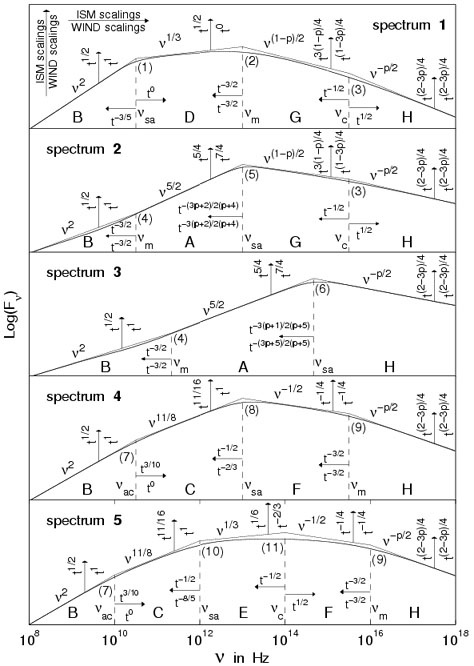Figure 23. The different possible broad band synchrotron spectra from a relativistic blast wave, that accelerates the electrons to a power law distribution of energies. The thin solid line shows the asymptotic power law segments, and their points of intersection, where the break frequencies, b, and the corresponding flux densities, Fb, ext, are defined. The different PLSs are labelled A through H, while the different break frequencies are labelled 1 through 11. The temporal scalings of the power law segments and the break frequencies, for an ISM (k = 0) or stellar wind (k = 2) environment, are indicated by the arrows. The different spectra are labelled 1 through 5, from top to bottom. The relevant spectrum is determined by the ordering of the break frequencies. The top two panels (spectra 1 and 2) correspond to slow cooling (m < c). Spectrum 1 applies when sa < m, while spectrum 2 applies when m < sa < c. The two bottom panels (spectra 4 and 5) correspond to fast cooling (c < m). Spectrum 5 applies when sa < c, and spectrum 4 applies when c < sa < m. Spectrum 3 (middle panel) applies when sa > m, c, where in this case the relative ordering of c and m is unimportant (i.e. spectrum 3 may apply both to slow cooling or fast cooling). From [144].

These results are valid only for p > 2 (and for _max, the maximal electron energy, much higher than _min). If p < 2 then _max plays a critical role. The resulting temporal and spectral indices for slow cooling with 1 < p < 2 are given by Dai and Cheng [64] and by Bhattacharya [28] and summarized in table III below. For completeness I include in this table also the cases of propagation into a wind (see Section VIIE) and a jet break (see Section VIIH).

Table III. for slow cooling (_a < _m < _c) into a constant density ISM, wind and jet for electron distribution with 1 < p < 2.

	ISM	wind	Jet
< a	(17p-26)/16(p-1)	(13p-18)/18(p-1)	3(p-2)/4(p-1)
a < < m	(p+1)/8(p-1)	5(2-p)/12(p-1)	(8-5p)/6(p-1)
m < < c	-3(p+2)/16	-(p+8)/8	-(p+6)/4
c <	-(3p+10)/16	-(p+6)/8	-(p+6)/4

The simple solution, that is based on a homogeneous shell approximation, can be modified by using the full BM solution and integrating over the entire volume of shocked fluid [140]. Following [271] I discuss Section VIIG1 a simple way to perform this integration. The detailed integration yields a smoother spectrum and light curve near the break frequencies, but the asymptotic slopes, away from the break frequencies and the transition times, remain the same as in the simpler theory. Granot and Sari [144] describe a detailed numerical analysis of the smooth afterglow spectrum including a smooth approximation for the spectrum over the transition regions (see also [148]). They also describe additional cases of ordering of the typical frequencies which were not considered earlier.

A final note on this "standard" model is that it assumes adiabaticity. However, in reality a fraction of the energy is lost and this influences over a long run the hydrodynamic behavior. This could be easily corrected by an integration of the energy losses and an addition a variable energy to Eq. 74, followed by the rest of the procedure described above [290].

⁶ The following notation appeared in the astro-ph version of [376]. Later during the proofs that author realized that is used often in astrophysics to denote a spectral index and in the Ap. J. version of [376] the notations have been changed to F t^{- -}. However, in the meantime the astro-ph notation became generally accepted. I use these notations here. Back.