


In this Section, we briefly report selected results of the described projects. We describe very general observational results on the mean characteristics of galaxies.
Over many years, galaxy counts, i.e., the plot of the observed number of galaxies at the limiting magnitude, have been considered to be an important cosmological test. In particular, in the 1930s, Hubble tried to apply them to estimate the curvature of space. It became clear later that practical application of this test is so difficult (photometric errors, the account for k-correction, the evolution of galaxies with time) that "any attempt to do so appears to be a waste of telescope time" [87]. Presently, deep counts are regarded not as a cosmological test but rather as a test of galaxy formation and evolution.
Figure 11 summarizes modern results of
differential galaxy counts according to data from the web page
http://star-www.dur.ac.uk/~nm/pubhtml/counts/counts.html.
Only data obtained after 1995 are shown. With each filter, the
results of about twenty projects (including 2MASS, SDSS, HDF, CDF,
NDF, etc.) are summarized; with filter B, counts in the SDF,
VVDS, and HUDF fields are added. The figure shows good
agreement between the results of different works. For
example, for B 25m, the count dispersion is only about
10% (accounting for the photometry, different selection of
galaxies, etc., this dispersion must be even smaller), which
clearly illustrates the homogeneity and isotropy of large-scale
galaxy distribution. For brighter (and, on average, closer)
objects, the count dispersion increases due to large-scale
structure effects. The weakest source counts strongly suffer
from photometric errors and other factors.
25m, the count dispersion is only about
10% (accounting for the photometry, different selection of
galaxies, etc., this dispersion must be even smaller), which
clearly illustrates the homogeneity and isotropy of large-scale
galaxy distribution. For brighter (and, on average, closer)
objects, the count dispersion increases due to large-scale
structure effects. The weakest source counts strongly suffer
from photometric errors and other factors.
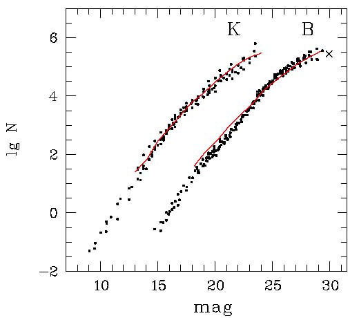 |
Figure 11. Differential counts of galaxies (the number of galaxies within a given range of apparent magnitudes normalized to 1 square degree) with filters B and K (dots). Data in filters B and K are calculated using 0.5m and 1.0m intervals, respectively. The cross marks the HUDF galaxy counts. The solid lines show predictions of the galaxy formation model in [88]. |
The solid lines in Fig. 11 show predictions of a semianalytic model of galaxy formation [88] (the `LC' model in that paper). Both this and other models (see, e.g., [89] and the references therein) can satisfactorily fit observations. However, the model predictions are not fully definitive due to many parameters characterizing galactic properties and their evolution with z (including spatial density evolution). For further progress in this field, both observational data and theoretical understanding of galaxy evolution must be improved.
The distribution of galaxies in the nearby volume of the Universe is highly inhomogeneous (Figs 3, 4). When passing to the hundred Megaparsec scale, the density fluctuations smoothen and the distribution becomes more homogeneous (Fig. 5).
The clustering of galaxies is usually described in terms of
two-point correlation functions
 (r) and
 (
( ).
The former function describes the joint probability of finding two
galaxies separated by a distance r, and the latter characterizes
the joint probability of detecting two objects at the angular
distance
[90].
To calculate
(r),
spatial distances between galaxies should be known, and in practice it
is therefore more convenient to measure the (angular) two-point correlation
function (). From
(), one can then estimate
(r)
because both functions are related through the Limber integral
equation. If
(r) can be
represented as a power law
(r)
= (r / r0)-
).
The former function describes the joint probability of finding two
galaxies separated by a distance r, and the latter characterizes
the joint probability of detecting two objects at the angular
distance
[90].
To calculate
(r),
spatial distances between galaxies should be known, and in practice it
is therefore more convenient to measure the (angular) two-point correlation
function (). From
(), one can then estimate
(r)
because both functions are related through the Limber integral
equation. If
(r) can be
represented as a power law
(r)
= (r / r0)- , the
angular correlation also takes
a power-law form ()
, the
angular correlation also takes
a power-law form ()
 1-
[90].
1-
[90].
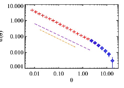
Figure 12 plots the angular correlation
function for ~ 0.5 million galaxies from the 2MASS survey
[91].
At angular scales 1' <
< 2.5°, this
function is well fit by a power law with
1- =
-0.79 ± 0.02. The amplitude
of () depends on the sample depth
- for brighter and closer objects, the clustering amplitude increases
(this, in particular, explains the systematic shift between different
survey data in Fig. 12).
 |
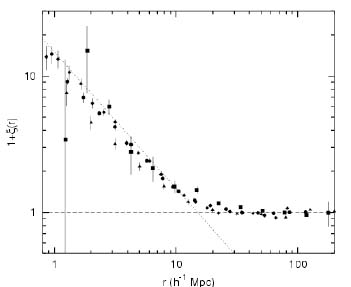 |
Figure 12. Top: the two-point angular
correlation function
|
In the bottom part of Fig. 12, we show the
correlation function
(r)
calculated in different papers (h in the figure
means the Hubble constant value expressed in units of
100 km/s/Mpc). In the range 0.1 Mpc
 r
20 Mpc,
this function follows a power law with the exponent
1.7-1.8, and then
tends to zero. The characteristic clustering scale (correlation length)
r0 for nearby galaxies is
7 Mpc. The
correlation length depends on the properties of
galaxies, such as their luminosity and morphological type (see, e.g.,
[93]),
but is independent of the sample depth (see the discussion in
[92]).
r
20 Mpc,
this function follows a power law with the exponent
1.7-1.8, and then
tends to zero. The characteristic clustering scale (correlation length)
r0 for nearby galaxies is
7 Mpc. The
correlation length depends on the properties of
galaxies, such as their luminosity and morphological type (see, e.g.,
[93]),
but is independent of the sample depth (see the discussion in
[92]).
Modern survey data allow determining the density fluctuations in the Universe as a function of the scale of averaging (Fig. 13). (The power spectrum of the SDSS galaxies, which has been used to plot this figure, is based on data on 2 × 10⁵ galaxies [95].) Figure 13 shows that different kinds of data, from galaxy density fluctuations to cosmic microwave background anisotropy, form a unique smooth dependence described by the CDM model.
 |
Figure 13. Density fluctuations
|
Recently completed surveys have allowed features of the
nearby galaxy distribution to be studied in a detail unavailable
earlier. In particular, the 2MASS survey enabled
examining the galaxy distribution in the `zone of avoidance'
- the strip near the Milky Way plane (|b| < 10°) where the
interstellar absorption screens extragalactic objects
[96].
The galaxy distribution as derived from the 2MASS, 2dF, and
APM surveys led to the conclusion that there is a 30% deficit
of bright galaxies in the southern galactic hemisphere in
comparison with the northern one
[97].
The authors believe
that the observed deficit is a consequence of a huge `hole' with
a linear size possibly exceeding 200 Mpc in the local galaxy
distribution. Such a large local nonhomogeneity, as well as
the possible presence of a well-defined large-scale structure at
z ~ 6
([66],
see Section 4.5;
[98]),
can pose certain problems
for the standard CDM model. We note that nonhomogeneities
of a comparable scale ( 200 Mpc) have been found in the quasar distribution derived from the 2QZ
project (see Section 3.5)
[99].
200 Mpc) have been found in the quasar distribution derived from the 2QZ
project (see Section 3.5)
[99].
5.3. Evolution of the luminosity function
The luminosity function (LF) is the dependence of the number of galaxies within a unit volume on their luminosity. It is one of the most important integral characteristics of galaxies. The LF allows estimating the mean luminosity density in the Universe. The LF form is one of the main tests of galaxy formation models. The standard form of the LF is the so-called Schechter function [100]
 |
where  (L)
dL is the number of galaxies with the luminosity
from L to L + dL per unit volume, and
*, L* and
(L)
dL is the number of galaxies with the luminosity
from L to L + dL per unit volume, and
*, L* and
 are parameters. The
parameter * yields the
normalization of the LF, L* is the
characteristic luminosity,
and determines
the slope of the weak wing (L <
L*) of the LF: the weak wing
of the LF is flat for =
-1, the LF increases with decreasing
L for < -1,
and decreases at >
-1. The Schechter function fits well the real LF of field galaxies and
clusters and has convenient analytical properties.
are parameters. The
parameter * yields the
normalization of the LF, L* is the
characteristic luminosity,
and determines
the slope of the weak wing (L <
L*) of the LF: the weak wing
of the LF is flat for =
-1, the LF increases with decreasing
L for < -1,
and decreases at >
-1. The Schechter function fits well the real LF of field galaxies and
clusters and has convenient analytical properties.
At present, the local LF of galaxies is relatively
well studied. According to many papers (including the 2dF
and SDSS surveys), within the absolute magnitude range
-15m
M(B)
-22m (filter B), the LF can be described
with the following values of parameters:
-(1.1-1.2),
M*(B)
-20.2m
(L*(B) = 1.9 × 10¹⁰
L ,B), and
*
(0.5-0.7) × 10-2 Mpc-3 (see. e.g.,
[101]).
Therefore, the luminosity density of galaxies at z = 0 is
 L(B) =
* L*
L(B) =
* L*
 ( + 2)
1.3 × 10⁸
L,B
/ Mpc3
( + 2)
1.3 × 10⁸
L,B
/ Mpc3
and the galaxy density is
=
L
/ L* =
*
( + 2) ~ 10-2
Mpc-3.
The LF of local galaxies depends on their morphological type
and environment
[102].
Numerous deep field studies performed over the last ten
years have enabled the evolution of the LF with z to be
determined. In solving this problem, the so-called `photometric
redshifts' inferred from multicolor photometry are
used instead of spectroscopic ones for the most distant
objects. Such a photometry allows a kind of a low-resolution
spectrum and hence z of an object to be obtained. Photometric
estimations of z are being made with
10%-20%
accuracy, which is quite sufficient to derive the LF for large
samples of galaxies.
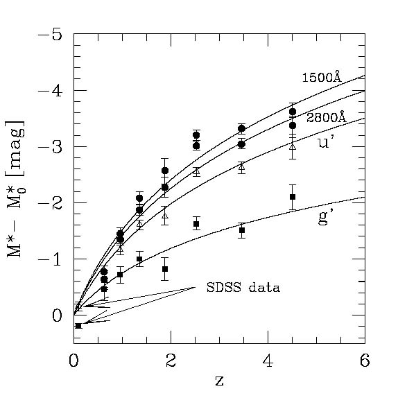
Observations suggest a differential (depending on the
galaxy type and the color band) evolution of the LF.
Different papers give somewhat different results, but the
qualitative picture emerging is as follows: the value of
M* increases with z, while
* decreases
(Fig. 14). According to
[103],
towards z ~ 5, the value of M* in
filter B increases by 1m-2m, and
* decreases by 5-10 times. The
evolution of the
LF slope is much less definitive, although some authors note a
decrease in with
z. By considering different types of objects
separately, the space density of elliptical and early spiral
galaxies almost stays constant or slightly decreases toward
z~ 1, while their LF evolution can be described as a change in
the luminosity of galaxies (they become brighter). In contrast,
the space density of late spiral galaxies with active star
formations notably increases toward z ~ 1
[104,
105].
The change in the LF of galaxies alters the luminosity density they
produce: from z = 0 to z ~ 3, the value of
L
increases, with the strongest growth being in the UV region (by about 5
times
[106]).
 |
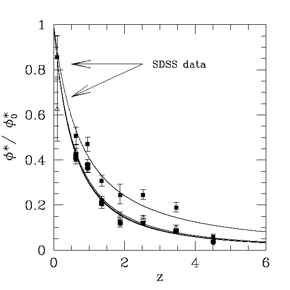 |
Figure 14. The redshift dependence of the
parameters of the luminosity
function of galaxies M* (top) and
|
5.4. Evolution of the galaxy structure
One of the main goals of the deep field galaxy studies is the origin and evolution of the Hubble sequence. In the local Universe, the optical morphology of the vast majority of bright galaxies can be described in terms of a simple classification scheme suggested by Hubble [3]. Only about 5% of nearby objects do not fit this scheme and are related to irregular or interacting galaxies [107, 108].
The deep HST fields for the first time allowed us to see the structure of distant galaxies. The very first studies revealed that the fraction of galaxies that do not fit the Hubble scheme increases for fainter objects [109]. At z ~ 1 (where the age of the Universe is about half the Hubble time), the fraction of such galaxies reaches 30%-40% (see examples in Figs 6 and 9). The lack of a convenient classification for distant galaxies stimulated the development of new methods for analyzing their images and the construction of objective classification schemes invoking the characteristics such as asymmetry and concentration indices (see, e.g., [109, 110]).
The statistics of objects in some deep fields also suggests
that the fraction of interacting galaxies and merging galaxies
increases with z. With the (1 + z)m growth
assumed, observational data suggest m
2-4 for z ~ 1
[111,
112].
The evolution of the merging rate is likely to depend on the
mass of galaxies - it is most pronounced for massive objects
[112].
It is much more difficult to draw definitive conclusions on
the structure evolution for objects at z
1 due to the
increasing effects of the k-correction, the cosmological
diming of surface brightness and degradation of the resolution
[113].
The history with bar studies for distant galaxies
may serve as an instructive illustration. The first morphological
studies of galaxies in the HDF implied a drastic decrease
in the fraction of barred spirals at z > 0.5, but the subsequent
analysis indicated that this fraction remains almost constant
(~ 40%), at least up to z = 1.1
[114,
115].
A significant amount of observational data has been
obtained about changes in the characteristics of large-scale
subsystems of galaxies. For example, it has been established
that by z ~ 1, the disk surface brightness of spiral galaxies
increases by ~ 1m, while the color indices decrease (i.e.,
become `bluer')
[116,
117].
For z 1, a change in
the slope of
the Tully-Fisher relation is found (the Tully-Fisher relation
is the dependence between the maximum rotation velocity and
the luminosity of spiral galaxies)
[118].
This slope change is
believed to be a consequence of the differential evolution of
spiral galaxies: at z ~ 1, low-mass spirals become brighter by
1m - 2m, while massive ones stay virtually as
bright. Disks of
`edge-on' spirals at z ~ 1 show a larger relative thickness (the
ratio of the vertical and radial scales in the brightness
distribution) and demonstrate vertical deformations of the
plane (warps) more frequently than nearby objects
[119,
120].
Spectral studies of spiral galaxies suggest their chemical
composition evolution: from z = 0 to z = 1, the metallicity
of gas subsystems of galaxies decreases
[121].
Some papers have investigated photometric and kinematical characteristics of elliptical galaxies in the field and in clusters up to z ~ 1 (see, e.g., [122, 123]). A deviation of distant early-type galaxies from the Fundamental Plane determined by the nearby objects has been discovered. This deviation is explained by the so-called `passive' evolution of their luminosities and, correspondingly, the mass-luminosity ratio (see [40, 124] for more details).
5.5. The most distant galaxies
Searches for and studies of the most distant galaxies in the Universe are some of the most interesting and important fields of extragalactic astronomy. The most distant and hence the youngest galaxies provide invaluable tests of galaxy formation models and allow processes in the relatively early Universe to be studied.
The history of discoveries of the most distant galaxies is shown in Fig. 15. It is seen that quasars had been the most distant objects over almost three decades. (The term `quasar' itself had often served as a synonym for the most distant objects.) The explanation is simple, because quasars are associated, as a rule, with very bright galaxies whose spectra show powerful and wide emission lines. The brightness of quasars and lines in their spectra make them much easier to observe from cosmological distances than ordinary galaxies (for example, see the spectrum of a distant quasar in Fig. 16). At the beginning of the new millennium, new methods appeared that allowed a very effective selection of ordinary galaxies at high z; since then, these galaxies and not quasars have been the most distant known objects in the Universe (Fig. 15).
 |
Figure 15. The history of detection of the most distant objects in the Universe (the circles are for galaxies, the crosses are for quasars). Years when the objects were discovered are plotted along the horizontal axis. Along the vertical axis to the left are plotted redshifts, and to the right - time in billions of years since the beginning of the cosmological expansion. The plot relies on the data in review [125] added with data obtained in recent years. |
There are several methods of selecting galaxies at high z.
Analysis of broad-band color indices to find galaxies with
peculiar colors (see Section 2) is one
of the most effective means of selecting very distant galaxies. This
method is primarily aimed at searching for galaxies with an energy
distribution break near the Lyman continuum (912 Å),
which is expected in star-forming galaxies
[9].
Due to the absorption in
L clouds along the line
of sight, emissions in
the spectra of distant galaxies between 912 Å and the
L line
are absorbed. This creates an additional spectral feature that
allows distant galaxies to be selected by their broad-band
color indices. More than a thousand objects with z > 2.5 have
been selected using this method; they are commonly referred
to as Lyman-break galaxies or simply LBGs (see
[9]
for a detailed review).
The second method frequently used is the search for
galaxies showing a strong emission
L line using a deep
narrow-band photometry of individual areas of the sky
followed by a spectroscopic study of the detected objects
(see Section 2 for more
details). Objects found this way are
often called `L
emitters,' or LAEs. It is by using this method
that the most distant object known so far with z = 6.60 was
discovered and signs of the presence of a large-scale structure
of galaxies at z = 5.7 were found
(Section 4.5).
At present, more than thirty galaxies with spectroscopic z > 5 have been reliably detected [64, 128] (see an example of the spectrum in Fig. 16). The age of such objects does not exceed ~ 10% of the age of the Universe (Fig. 15). Distant galaxies have been discovered both in deep fields and near galaxy clusters enhancing fluxes from remote background galaxies due to gravitational lensing.
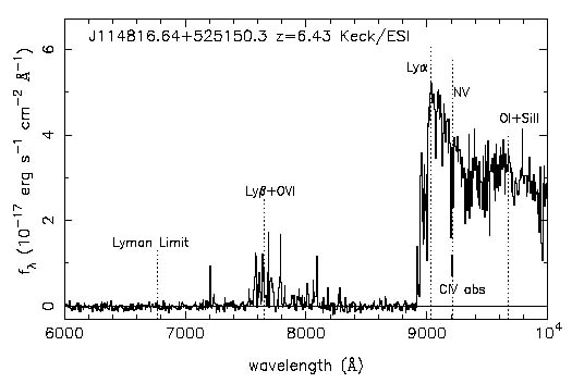 |
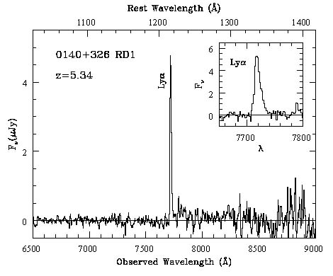 |
Figure 16. The spectrum of a quasar with z = 6.4 (top) [126] and the spectrum of a galaxy with z = 5.34 (bottom) [127]. |
The main observational features of galaxies with z > 5 (see, e.g.,
[64,
129])
are as follows:
- as a rule, morphologically peculiar, asymmetric,
compact shapes (the characteristic linear size is 1-5 kpc);
- a very high surface brightness and luminosity
(corrected for the cosmological brightness decrease and
k-correction effects);
- equivalent widths of the
L line in the comoving frame
are W(L) ~ 20-100
Å;
- the star formation rate inferred from the
L line luminosity is ~ 5-10
M/yr (this rate
estimated from the UV continuum luminosity is several times larger).
These characteristics are very strongly biased by the selection procedure itself, and it is therefore unclear to what extent they reflect actual properties of all objects located at z > 5. The observed objects can be `building blocks' that later merge and accrete the surrounding matter to form the galaxies we now know in our vicinity. On the other hand, some of these objects can represent bulges of massive spirals under formation or elliptical galaxies.
The clustering of LBGs and LAEs has been studied in
some papers. For bright galaxies (L
L*), the clustering scale
r0 does not show significant evolution from z =
0 to z = 5
[130,
131].
In contrast, the `bias parameter' b characterizing
the difference in space distribution of galaxies and dark halos
increases several times toward z = 5
[131].
The GOODS and
HUDF results may indicate an evolution in galaxy sizes: from z ~
2 to z ~ 6, the mean linear sizes decrease by about two times
[132,
133].
Both the galaxy clustering evolution and
change in the galaxy sizes can be explained by the CDM
model of galaxy formation.
The spectra of the most distant galaxies and quasars
provide the possibility of studying an early evolution of the
intergalactic medium. In particular, the so-called Gunn-Peterson effect
[134]
(a trough in the spectra of distant
objects shorter than L
due to absorption by neutral
hydrogen clouds along the line of sight) allows estimating the
redshift at which the secondary ionization epoch (re-ionization)
of the Universe has been completed
[135].
The discovery of this effect in spectra of quasars with z > 6
(Fig. 16) and its
absence for objects with z
6 suggest the
re-ionization epoch
(i.e., ionization of the intergalactic medium by radiation from
star formation regions and active galactic nuclei) to have been
completed by z ~ 6
[136,
126].
On the other hand, the cosmic
microwave background anisotropy measurements may evidence the
beginning of secondary ionization at z ~ 20 (see,
e.g., review
[137]).
The combination of these data has led to
the conclusion of a complicated, possibly two-stage, history
of the secondary ionization of the intergalactic medium
[138].
5.6. History of star formation in the Universe
Reconstruction of the global history of star formation in the Universe from z ~ 6 until now appears to be one of the most intriguing results derived in recent years from sky surveys and deep fields. Quantitative results by different authors are somewhat different, but the general trend of star formation in the unitary comoving volume as a function of redshift, which is often referred to as the `Madau diagram/plot' [139], is likely to be firmly established (see, e.g., Fig. 17).
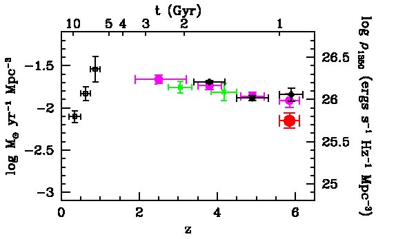 |
Figure 17. The history of star formation in
the Universe
[140].
The specific star formation rate in units
M |
There are two approaches to constructing this plot. The first relates to a detailed modeling of the star formation history in nearby galaxies using their spectra. The second is more direct and assumes studies of complete samples of galaxies observed at different z. The main problems of this method are relatively small samples of distant galaxies (which is related to the small sizes of deep fields) and poorly known correction for the intrinsic absorption, which can notably reduce the observed luminosity of distant objects. Nevertheless, both approaches yield generally consistent results (see, e.g., [141]).
As seen in Fig. 17, the specific star formation
rate rapidly grows from z = 0 to z ~ 1, has a global
maximum at z ~ 1-2,
and then starts decreasing, remaining, however, significant up
to the limiting redshift z (~ 6) at which modern estimates are
possible. Analysis of the history of star formation in the
Universe leads to the conclusion that 50% of all stars existing
at z = 0 were born at z
1, ~ 25% appeared at
z 2,
~ 15% appeared at z
3, and ~ 5% existed already at z = 5
[142].
One more important observational result is that the number
of massive star systems (with masses exceeding 1011
M)
decreases with z, although a small number of such galaxies
are also present at z > 4
[142].

 = 1350 Å is
plotted to the right. The upper horizontal axis plots the time since
the beginning of the cosmological expansion.
= 1350 Å is
plotted to the right. The upper horizontal axis plots the time since
the beginning of the cosmological expansion.