2. OBSERVED SOURCE COUNTS

2.1. From surveys to counts

The counts of sources demand cosmic evolution, but by themselves provide limited information on this evolution. Since even bright radio sources are frequently optically faint to invisible, the traditional way to characterize the evolutionary properties relies heavily on source counts from blind surveys, with limited and incomplete cross-waveband identification and redshift information. However, as discovered in the 2C survey, getting from a sky survey to a source count is difficult, and modern instrumentation, while generally avoiding the confusion issue which bedevilled 2C, does not remove the difficulties.

It is surface brightness, or rather differential surface brightness above a background (CMB, Galactic radiation, ground radiation), which is measured in radio/mm surveys. Discrete sources stand out from this background by virtue of apparent high differential surface brightness, T_b. The simple relations linking T_b to point-source flux density (via the Rayleigh-Jeans approximation and the radiometer equation incorporating telescope and receiver parameters) appear in basic radio astronomy texts, e.g Burke & Graham-Smith (1997).

Surveys are complete only to a given limit in T_b, translating to Jy per beam area ². For point sources, this limit is clearly defined. For extended sources, the total flux density

(1)

i.e. the incremental brightness B must be integrated over the extent of the source to find the total flux density. If a source is extended and its brightness temperature is constant across the beam response, then given the Rayleigh-Jeans approximation B = 2k_b T_b / ² (k_b is the Boltzmann constant, is wavelength), for a survey sensitivity limit of S_lim per beam, we have from eq. (1)

(2)

The integral is the beam solid angle; for a circular Gaussian beam with full width at half maximum of FWHM arcsec, this may be approximated as 2.66 × 10^-11 FWHM² sterad. Two iconic sky surveys at 1.4 GHz with the NRAO Very Large Array illustrate the brightness limit issue. For the FIRST survey (Becker et al. 1995) with FWHM = 5 arcsec and S_min = 1 mJy, eq. (2) gives T_min 24 K, while for the NVSS survey (Condon et al. 1998) with a 45 arcsec beam and S_min = 3 mJy, T_min 0.9 K. There are significant selection effects which arise as a consequence, most notably the lack of sensitivity in FIRST to the majority of spiral galaxies, near and far, as well as to low surface brightness features such as ghost or relic radiation. The redeeming features of its higher resolution are emphasized below.

It is a major undertaking to proceed from a list of deflections in Jy per beam, either apparently unresolved, or resolved as regions of emission, to a complete catalogue of radio/mm sources. In the first place, there is the surface brightness limitation described above; in the compromises of survey design it is critical to decide just what population(s) of sources will be incompletely represented. There is the issue of overlap: for instance Centaurus A, NGC 5128, the nearest canonical radio galaxy, extends over 9 degrees of the southern sky; there are many discrete distant sources catalogued within the area covered by Cen A. There is also the double nature of radio-galaxy emission: this requires that components found as individual detections be `matched up' or assembled to find the true flux density of single sources, cores as well as double lobes. Moreover many sources show extended regions of lower surface brightness which are poorly aligned. If source scale is large enough, pencil-beam or filled aperture telescopes are better at finding and mapping these than are aperture-synthesis interferometers. The issue of `missing flux' is notorious for interferometers, because of their limited response to the longer wavelengths of the spatial Fourier transform of the brightness distribution.

The difficulties have been brought to sharp focus by the excellent decision to carry out the two major VLA surveys, FIRST (Becker et al. 1995) and NVSS (Condon et al. 1998), both at 1.4 GHz but differing in resolution by a factor of 9. From these highly complementary surveys, the reality of how different resolutions affect raw source lists may be seen immediately (Blake & Wall 2002b). FIRST and NVSS are far more than the sum of the parts. The low resolution of NVSS gains the spiral galaxies and much other low-surface-brightness detail not seen in FIRST. The relatively high resolution of FIRST can be used to sort out the blends and overlaps in NVSS, and it enables direct cross-waveband identifications, a shortcoming of the lower NVSS resolution. Used together they can provide samples complete on many criteria; but significant effort in examining many individual emission features is still required.

With regard to surveys using interferometers, the noise level in an interferometric image is given by:

(3)

where T_sys is the system temperature, A is the antenna surface area, _e is the aperture efficiency, the ratio of effective collecting area to surface area, _q is the sampling efficiency depending on digitization levels and sampling rate, t is the integration time, N_base = N(N - 1)/2 is the number of baselines, N is the number of antennas, and is the bandwidth. (_e is generally 0.3 to 0.8, and _q 0.7 to 0.9.) The integration time per pointing needed to reach a detection limit of say S_lim = 5_image can be straightforwardly obtained from eq. (3). The number of pointings necessary to cover a sky solid angle _s with a telescope field of view FOV is ³

(4)

If the integral counts of sources scale as S^-, the number of sources detected in a given area scales as t^/2. For a given flux density, the number of detections is proportional to the surveyed area, i.e. to t. Thus, to maximize the number of detections in a given observing time it is necessary to go deeper if > 2 and to survey a larger area if < 2. The `narrow and deep' vs. `wide and shallow' argument for maximizing source yield always resolves, at radio frequencies, in favour of the latter, because > 2, implying a differential count slope of less than -3, has never been observed at any flux-density level. On the other hand, very steep counts are observed at millimeter and sub-millimeter wavelengths (Austermann et al. 2009, Coppin et al. 2006).

Compilation of complete and reliable catalogues, complete samples, almost invariably involves data at other frequencies. Source-component assembly for example is an iterative process which may require cross-waveband identification of the host object, galaxy, quasar, etc. The identification process leads on to the construction of complete samples, complete at both the survey frequency and at some other wavelength, i.e. in optical/IR identifications. Such samples are rare and require great observational effort. One of the best known of these, the '3CRR' sample (Laing et al. 1983) is a revised version of the revised 3C catalogue (Bennett 1962) from the original 3C survey of (Edge et al. 1959). (The sample is also the most extreme sample of high-power radio AGN, and its contents are far from typical of the radio-mm survey population.) The process will become easier with large-area optical surveys such as SDSS (York et al. 2000) and with the advent of synoptic telescopes such as LSST.

Given complete samples, then, we can compile source counts. (It should be noted that these are frequently constructed by approximations from raw deflection lists, to circumvent the labour discussed above. Caveat emptor. ⁴) Today the task of checking for systematic effects from approximations or statistical procedures is made easier because the counts from different survey samples - except for the very deepest ones - overlap at various flux-density levels. The counts are usually presented in `relative differential' form, the differential counts dN / dS giving the number of sources per unit area with flux density S within dS, subsequently and conveniently normalized to the 'Euclidean' form, i.e. multiplied by cS^2.5, with c being a suitably chosen constant. (A uniform source distribution in a static Euclidean universe yields dN / dS S^-2.5 as described earlier). A summary of the available source counts at different frequencies is given in Tables 1 - 10 (see also Figs. 5-7).

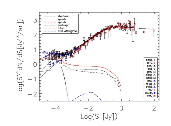Figure 5. Normalized differential source counts at 1.4 GHz. Note that the filled diamonds show the counts of AGNs only, while all the other symbols refer to total counts. Reference codes are spelt out in the note to Table 5. A straightforward extrapolation of evolutionary models fitting the far-IR to mm counts of populations of star-forming (normal late type (spirals or sp), starburst (sb), and proto-spheroidal) galaxies, exploiting the well established far-IR/radio correlation, naturally accounts for the observed counts below ~ 30 µJy (see Section 6). At higher flux densities the counts are dominated by radio-loud AGNs: the thick solid line shows the fit of the same model as in Fig. 4. The dot-dashed line shows the counts of -ray burst (GRB) afterglows predicted by the (Ciardi & Loeb 2000) model.

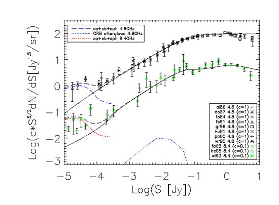Figure 6. Differential source counts at 4.8 and 8.4 GHz normalized to c × S-2.5, with c = 1 and 0.1, respectively. Reference codes are spelt out in the notes to Tables 6 and 7. In the upper inset sp, sb, and sph stand for spiral, starburst and proto-spheroidal galaxies, respectively. The fit to the 4.8 GHz counts is from the same model as in Figs. 4 and 5, while at 8.4 GHz we show the fit yielded by the De Zotti et al. (2005) model, tailored for data above 5 GHz. The dotted line shows the counts of GRB afterglows at 3 GHz predicted by the Ciardi & Loeb (2000) model.

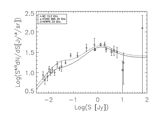Figure 7. Differential source counts normalized to S-2.5 for the 15 GHz 9C survey (Waldram et al. 2003, Waldram et al. 2009), for the 20 GHz ATCA Bright Source Sample (Massardi et al. 2008a), and for the WMAP 23 GHz survey (Massardi et al. 2009). The model by De Zotti et al. (2005) is also shown for comparison (solid line: 20 GHz, dotted: 15 GHz).

In the case of surveys covering small areas, the field-to-field variations arising from the source clustering (sampling variance) further adds to the uncertainties. The fractional variance of the counts is (Peebles 1980):

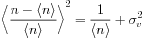(5)

with

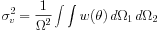(6)

where is the angle between the solid angle elements d₁ and d₂, and the integrals are over the solid angle covered by the survey.

The angular correlation function of NVSS and FIRST sources (see Section 9) is consistent with a power-law shape (Blake & Wall 2002a, Blake & Wall 2002b, Overzier et al. 2003):

(7)

for angular separations up to at least 4°. Inserting eq. (7) in eq. (6) we get

(8)

The errors given in Tables 1 - 7 include this contribution for surveys over areas 25 deg².

Differences between source counts for independent fields are in general far larger than these errors imply (Condon 2007). There is little doubt that different calibrations, beam corrections and resolution corrections are the dominant if not exclusive culprits. Further advances in calibration procedures and characterization of the structures of faint sources will be required before sampling variance comes to dominate the errors in faint counts of radio sources.

2.2. Low frequency surveys

Low-frequency surveys have a long and illustrious (but initially chequered) history, as we have mentioned. The most extensive ones, both in terms of area (see also Section 9) and of depth, are those at ~ 1 GHz and at ~ 5 GHz. The NRAO VLA Sky Survey (NVSS; Condon et al. 1998) covers the sky north of = -40° (82% of the celestial sphere) at 1.4 GHz, down to ~ 2.5 mJy. It has resolution of 45 arcsec FWHM and the raw catalogue contains 1.8 × 10⁶ entries. It is complemented by the Sydney University Molonglo Sky Survey (SUMSS; Mauch et al. 2003) at 0.843 GHz. The survey was completed in 2007 with the Molonglo Galactic Plane Survey (MGPS; Murphy et al. 2007), and now covers the whole sky south of declination -30°.

The VLA 1.4-GHz FIRST survey (for Faint Images of the Radio Sky at Twenty-cm; Becker et al. 1995) is the high-resolution (5 arcsec FWHM) counterpart of NVSS, and has yielded accurate (< 1 arcsec rms) radio positions of faint compact sources. The new catalog, released in July 2008 (format errors corrected in October 2008), covers ~ 8444 deg² in the North Galactic cap and 611 deg² in the south Galactic cap, for a total of 9055 deg² yielding a list of ~ 816,000 objects. Northern and Southern areas were both chosen to coincide approximately with the area covered by the SDSS. The typical flux density detection threshold of point sources is of about 1 mJy/beam, decreasing to 0.75 mJy/beam in the southern Galactic cap equatorial stripe.

Almost full-sky coverage was also achieved at ~ 5 GHz - albeit to a much higher flux-density level - by the combination of the Northern Green Bank GB6 survey with the Southern Parkes-MIT-NRAO (PMN) survey. The GB6 catalog (Gregory et al. 1996) covers the range 0° 75° down to ~ 18 mJy/beam, the FWHM major and minor diameters are of 3'.6 and 3'.4, respectively. The flux-density limit of the PMN catalog (Griffith & Wright 1993) is typically ~ 30 mJy/beam but varies with declination, which spans the range from -87.5° to +10°; the FWHM is of 4'.2.

Other large-area, low-frequency surveys:

• the VLA Low-Frequency Sky Survey (VLSS; Cohen et al. 2007) is a 74-MHz continuum survey covering the entire sky North of = -30° to a typical point-source detection limit of 0.7 Jy.

• the Cambridge 6C survey at 151 MHz (Hales et al. 1993 and references therein) covers most of the extragalactic sky above = 30°, but generally away from the Galactic plane, with 4.2' × 4.2' csc resolution. The 7C survey (Hales et al. 2007), at the same frequency, covers a similar region of the sky with higher resolution (70'' × 70'' csc()). A somewhat lower-resolution survey has been carried out in the low-declination strip 9h < RA < 16h, 20°< < 35° (Waldram et al. 1996).

• The 8C survey (Rees 1990, Hales et al. 1995) covers the polar cap above = 60° at 38 MHz with a typical limiting flux density of about 1 Jy/beam.

• The Westerbork Northern Sky Survey (WENSS; Rengelink et al. 1997, de Bruyn et al. 2000) covers the 3.14 sr north of = +30° at 326 MHz with 54'' × 54''csc() resolution in total intensity and linear polarization, to a flux-density limit of approximately 18 mJy/beam.

For more complete references to low-frequency radio surveys, see Tables 1 - 7.

2.3. Deep surveys and sub-mJy counts

The deepest surveys cover small areas of sky on the scales of the primary beams of synthesis telescopes; they are carried out with such telescopes in single long exposures, or in nested overlapping sets of such exposures. Because source counts are steep, only small survey areas are required to obtain large enough samples of faint sources to be statistically significant.

From such surveys, the deepest counts at 1.4 to 8.4 GHz show an inflection point at 1 mJy (Mitchell & Condon 1985, Windhorst et al. 1985, Hopkins et al. 1998, Richards 2000, Bondi et al. 2003, Ciliegi et al. 2003, Hopkins et al. 2003, Seymour et al. 2004, Huynh et al. 2005, Prandoni et al. 2006, Fomalont et al. 2006, Simpson et al. 2006, Bondi et al. 2007, Ivison et al. 2007, Bondi et al. 2008, Owen & Morrison 2008). The point of inflection was originally interpreted as signalling the emergence of a new source population (e.g. Condon 1984a, Condon 1989). Windhorst et al. (1985) suggested that the majority of sub-mJy radio sources are faint blue galaxies, presumably undergoing significant star formation (SF), and Danese et al. (1987) successfully modeled the sub-mJy excess counts with evolving starburst galaxies, a model that also described the IRAS 60 µm counts.

More recent data and analyses have confirmed that starburst galaxies are indeed a major component of the sub-mJy 1.4 GHz source counts, perhaps dominating below 0.3-0.1 mJy (Benn et al. 1993, Rowan-Robinson et al. 1993, Hopkins et al. 1998, Hopkins et al. 2000, Seymour et al. 2004, Seymour et al. 2008, Muxlow et al. 2005, Moss et al. 2007, Padovani et al. 2009). However, spectroscopic results by Gruppioni et al. (1999b) suggested that early-type galaxies were the dominant population at sub-mJy levels. Further, it was recently suggested (and modeled) that the flattening of the source counts may be caused by 'radio-quiet' AGN (radio-quiet quasars and type 2 AGN), rather than star forming galaxies (Simpson et al. 2006). Distinct counts for high and low-luminosity radio galaxies show that low-luminosity FRI-type galaxies probably make a substantial contribution to the counts at 1 mJy and somewhat below (Gendre & Wall 2008). Based on a combination of optical and radio morphology as an identifier for AGN and SF galaxies, Fomalont et al. (2006) suggested that at most 40% of the sub-mJy radio sources are AGNs, while Padovani et al. (2007b) indicated that this fraction may be 60-80%. Huynh et al. (2008) found that the host galaxy colors and radio-to-optical ratios indicate that low-luminosity (or "radio-quiet") AGN make up a significant proportion of the sub-mJy radio population. Smolcic et al. (2008), using a newly developed rest-frame-colour based classification in conjunction with the VLA-COSMOS 1.4 GHz observations, concluded that the radio population in the flux-density range of ~ 50 µJy to 0.7 mJy is a mixture of 30-40% of star forming galaxies and 50-60% of AGN galaxies, with a minor contribution (~ 10%) of QSOs.

The origin of these discrepancies can be traced to three main reasons (see also Section 3). First, the identification fraction of radio sources with optical counterparts, which is generally taken to be representative of the full radio population, spans a wide range (20% to 90%) in literature depending on the depth of both the available radio and optical data. Second, it is important to make a distinction between the presence of an AGN in the optical counterpart of a radio source, and its contribution to the radio emission (Seymour et al. 2008). Non-radio AGN indicators like optical/IR colours, emission lines, mid-IR SEDs, X-ray emission, etc. are not well correlated with the radio emission of the AGNs and therefore are not necessarily valid diagnostics of radio emission powered by accretion onto a supermassive black hole (Muxlow et al. 2005). Third, there are uncertainties in specifying survey level: deep surveys normally cover but one primary beam area, heavily non-uniform in sensitivity. A survey claimed complete at some specified flux density in the central region alone is in fact heavily biased to sources of 5 to 10 times this flux density; the survey as a result is biased to the higher-flux-density population, namely AGNs.

Seymour et al. (2008) used four diagnostics (radio morphology, radio spectral index, radio/near-IR and mid-IR/radio flux-density ratios) to single out, in a statistical sense, radio emission powered by AGN activity. They were able to calculate the source counts separately for AGNs and star-forming galaxies. The latter were found to dominate below 0.1 mJy at 1.4 GHz, while AGNs still make up around one quarter of the counts at ~ 50 µJy.

Bondi et al. (2008) pointed to evidence of a decline of the 1.4 GHz counts below ~ 0.1 mJy. It is possible that a new upturn may be seen at 1 µJy, due to the emergence of normal star-forming galaxies (Windhorst et al. 1999, Hopkins et al. 2000).

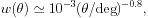
Essentially all surveys and catalogues are carried out and compiled without reference to polarization (the NVSS being an important exception): linear polarization is generally less than a few percent, and certainly at mJy levels, below the uncertainties in flux densities due to calibration, noise and confusion. An average of circular polarizations is generally used. (Subsequent to surveys, thousands of measurements of polarization on individual sources have been carried out at different frequencies, with the rotation measures thus derived used to map the details of the Galactic magnetic field - see e.g. Brown et al. 2007). The DRAO 1.4-GHz survey of the ELAIS N1 field (Taylor et al. 2007) was carried out expressly to examine polarization statistics. The data at the faintest flux densities, 0.5 to 1.0 mJy, show a trend of increasing polarization fraction with decreasing flux density, previously noted by Mesa et al. (2002) and Tucci et al. (2004), at variance with current models of population mix and evolution.

2.4. High frequency surveys and counts

High-frequency surveys up into the mm-wavelength regime vitally complement their low-frequency counterparts. The early cm-wavelength surveys (Parkes 2.7 GHz, NRAO 5 GHz) in the late 1960s and 1970s found that flat-spectrum sources - or at least sources whose integrated spectra were dominated by components showing synchrotron self-absorption - constitute 50% or more of all sources in high flux-density samples. Modelling space density to examine evolution demands determination of the extent and nature of this emergent population, most members of which are blazars.

High-frequency surveys are very time-consuming. For telescopes with diffraction-limited fields of view the number of pointings necessary to cover a given area scales as ². For a given receiver noise and bandwidth, the time per pointing to reach the flux level S scales as S^-2 so that, for a typical optically-thin synchrotron spectrum (S ^-0.7), the survey time scales as ^3.4. However usable bandwidth is roughly proportional to frequency, so that the scaling becomes ~ ^2.4; but a 20 GHz survey still takes more than ~ 25 times longer than a 5 GHz survey to cover the same area to the same flux-density limit.

High-frequency surveys have an additional aspect of uncertainty: variability. The self-absorbed components are frequently unstable, young and rapidly evolving. Variability by itself would not be an issue except for the fact that it leads to serious biases. This is primarily because a survey will always select objects in a high state at the expense of those in a low state, and the steep source count at high flux densities exacerbates this situation. A second issue concerns the spectra. Sources are predominantly detected `high'; to return after the survey for flux-density measurements at other frequencies guarantees (statistically) that these new measurements will relate to a lower state. Non-contemporaneous spectral measurements - if above the survey frequency - will be biased in the sense of yielding spectra apparently steeper than at the survey epoch. The bias can have serious consequences for e.g. K-corrections in space-density studies, as described below.

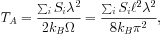
Cosmic Microwave Background (CMB) studies, boosted by the on-going NASA WMAP mission and by the forthcoming ESA Planck mission, require an accurate characterization of the high-frequency properties of foreground radio sources both in total intensity and in polarization. Radio sources are the dominant contaminant of small-scale CMB anisotropies at mm wavelengths. This can be seen by recalling that the mean contribution of unresolved sources with flux S_i to the antenna temperature T_a measured within a solid angle is:

(9)

where k_b is the Boltzmann constant, is the observing wavelength, and we have taken into account that for high multipoles ( >> 1), (2 / )². If sources are randomly distributed on the sky, the variance of T_a is equal to the mean, and their contribution to the power spectrum of temperature fluctuations grows as ² while the power spectra of the CMB and of Galactic diffuse emissions decline at large 's (small angular scales). Therefore, Poisson fluctuations due to extragalactic sources are the dominant contaminant of CMB maps on scales 30', i.e. 400 (De Zotti et al. 1999, Toffolatti et al. 1999).

The diversity and complexity of radio-source spectra, particularly for sources detected at the higher frequencies, make extrapolations from low frequencies, where extensive surveys exist, unreliable for the purpose of establishing CMB contamination. Removing this uncertainty was the primary motivation of the Ryle-Telescope 9C surveys at 15.2 GHz (Taylor et al. 2001, Waldram et al. 2003). These were specifically designed for source subtraction from CMB maps produced by the Very Small Array (VSA) at 34 GHz. The surveys have covered an area of 520 deg² to a 25 mJy completeness limit. (Waldram et al. 2009) reported on a series of deeper regions, amounting to an area of 115 deg² complete to approximately 10 mJy, and of 29 deg² complete to approximately 5.5 mJy. The counts over the full range 5.5 mJy - 1 Jy are well described by a simple power-law:

(10)

A 20-GHz survey of the full Southern sky to a limit of 50 mJy has been carried out by exploiting the Australia Telescope Compact Array (ATCA) fast-scanning capabilities (15° min^-1 in declination along the meridian) and the 8-GHz bandwidth of an analogue correlator. The correlator was originally developed for the Taiwanese CMB experiment AMiBA (Lo et al. 2001) but has been applied to three of the 6 22 m dishes of the ATCA. A pilot survey (Ricci et al. 2004, Sadler et al. 2006) at 18.5 GHz was carried out in 2002 and 2003. It detected 173 sources in the declination range -60° to -70° down to 100 mJy. The full survey was begun in 2004 and was completed in 2008. More than 5800 sources brighter that 45 mJy were detected below declination = 0°. An analysis of a complete flux-limited sub-sample (S_{20 GHz} > 0.50 Jy) comprising 320 extragalactic radio sources was presented by (Massardi et al. 2008a).

Shallow (completeness levels 1 Jy) all-sky surveys at 23, 33, 41, 61, and 94 GHz have been carried out by the Wilkinson Microwave Anisotropy Probe (WMAP). Analyses of WMAP 5-year data have yielded from 388 (Wright et al. 2009) to 516 (Massardi et al. 2009) detections. Of the latter, 457 are identified with previously-catalogued extragalactic sources, 27 with Galactic sources; 32 do not have counterparts in lower frequency all sky surveys and may therefore be just high peaks of the highly non-Gaussian fluctuation field.

Counts at ~ 30 GHz have been estimated from DASI data over the range 0.1 to 10 Jy (Kovac et al. 2002), from CBI maps in the range 5-50 mJy (Mason et al. 2003), and down to 1 mJy from the SZA blind cluster survey (Muchovej et al. 2009, in prep.).

Cleary et al. (2005) used 33-GHz observations of sources detected at 15 GHz to extrapolate the 9C counts in the range 20 mJy S₃₃ 114 mJy. Mason et al. (2009) carried out Green Bank Telescope (GBT) and Owens Valley Radio Observatory (OVRO) 31-GHz observations of 3165 NVSS sources; 15% of them were detected. 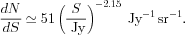Under the assumption that the S_{31 GHz} / S_{1.4 GHz} flux ratio distribution is independent of the 1.4 GHz flux density over the range of interest, they derived the maximum likelihood 1.4 to 31 GHz spectral index distribution, taking into account 31-GHz upper limits, and exploited it to estimate the 31-GHz source counts at mJy levels: N(> S) = (16.7 ± 0.4) deg^-2 (S / 1 mJy)^{-0.80 ± 0.01} (0.5 mJy < S < 10 mJy). The derived counts were found to be 15% lower than predicted by the De Zotti et al. (2005) model.

Preliminary indications of a spectral steepening of flat-spectrum sources above ~ 20 GHz, beyond the expectations of the blazar sequence model (Fossati et al. 1998, Ghisellini et al. 1998) have been reported. Waldram et al. (2007) used the spectral-index distributions over the range 1.4-43 GHz based on `simultaneous' multifrequency follow-up observations (Bolton et al. 2004) of a sample of extragalactic sources from the 9C survey at 15 GHz to make empirical estimates of the source counts at 22, 30, 43, 70, and 90 GHz by extrapolating the power-law representation of the 15-GHz counts (eq. (10)). Sadler et al. (2008) carried out simultaneous 20- and 95-GHz flux densities measurements for a sample of AT20G sources. The inferred spectral-index distribution was used to extrapolate the AT20G counts to 95 GHz. The extrapolated counts are lower than those predicted by the De Zotti et al. (2005) model, and (except at the brightest flux densities) also lower than the extrapolation by Holdaway et al. (1994) of the 5-GHz counts. On the other hand, they are within the range of the Waldram et al. (2007) estimates in the limited flux density range where both data sets are valid, although the slopes are significantly different. Both Waldram et al. (2007) and Sadler et al. (2008) assume that the spectral index distribution is independent of flux density. This can only be true for a limited flux density interval, since the mixture of steep-, flat-, and inverted-spectrum sources varies with flux density. In fact, the median 20-95 GHz spectrum ( = 0.39) found by Sadler et al. (2008) is much flatter than that ( = 0.89) measured at 15-43 GHz by Waldram et al. (2007) for a fainter sample.

Of course, extrapolations from low frequencies can hardly deal with the full complexity of source spectral and variability properties, and may miss sources with anomalously inverted spectra falling below the threshold of the low-frequency selection. They are therefore no substitute for direct blind high-frequency surveys. On the other hand, the recent high frequency surveys (9C, AT20G, WMAP) did not produce "surprises", such as a population of sources not present in samples selected at lower frequencies. The analysis of WMAP 5-yr data by Massardi et al. (2009) has shown that the counts at bright flux densities are consistent with a constant spectral index up to 61 GHz, although at that frequency there is a marginal indication of a spectral steepening. The WMAP counts at 94 GHz are highly uncertain because of the limited number of detections and the lack of a reliable flux calibration. However, taken at face value, the WMAP 94-GHz counts are below the predictions by the De Zotti et al. (2005) model by 30%. This indication is confirmed by recent measurements of the QUaD collaboration (Friedman & QUaD Collaboration 2009) who suggest that the model counts should be rescaled by a factor of 0.7 and of 0.6 at 100 and 150 GHz, respectively.

An indication in the opposite direction, albeit with very poor statistics, comes from the MAMBO 1.2-mm (250 GHz) blank-field imaging survey of ~ 0.75 deg² by Voss et al. (2006). This survey has uncovered 3 flat-spectrum radio sources brighter than 10 mJy, corresponding to an areal density several times higher than expected from extrapolations of low-frequency counts without spectral steepening.

A 43-GHz survey of ~ 0.5 deg², carried out with ~ 1600 snapshot observations with the VLA in D-configuration, found only one certain source down to 10 mJy (Wall et al., in preparation). A statistical analysis of the survey data yielded a source-count law in good agreement with predictions of Waldram et al. (2007) and Sadler et al. (2008). There is no strong indication of a previously unrecognized population intruding at this level.

² 1 Jy (Jansky) = 10^-26 W Hz^-1 m^-2 or 10^-23 erg cm^-2 s^-1 Hz^-1 Back.

³ This assumes uniform response over the field-of-view. The inevitable non-uniformity across the FOV implies an additional factor of ~ 2 for uniform sky coverage. The data from separate pointings are combined by squaring the relative response to weight the data by the square of the signal-to-noise ratio (SNR). If the beam is approximated by a Gaussian, then this process effectively halves the beam size; see Condon et al. (1998). Back.

⁴ The buyer should also beware of confusing as complete samples (a) lists of sources in which large volumes of data are assembled from different surveys and different completeness algorithms (e.g. PKSCat90, Wright & Otrupcek 1990), and (b) spectral samples, in which flux-density measurements at different frequencies are assembled to obtain the integrated spectra of samples of sources not necessarily selected by survey completeness (e.g. Pauliny-Toth et al. 1966, Kellermann et al. 1969). Back.