


Measurements of the two-point correlation function use the redshift of
a galaxy, not its distance, to infer its location along the line of
sight. This introduces two complications: one is that a cosmological
model has to be assumed to convert measured redshifts to inferred
distances, and the other is that peculiar velocities introduce
redshift space distortions in
 parallel to
the line of sight
(Sargent & Turner
1977).
On the first point, errors on the assumed
cosmology are generally subdominant, so that while in theory one could
assume different cosmological parameters and check which results are
consistent with the assumed values, that is generally not necessary.
On the second point, redshift space distortions can be measured to
constrain cosmological parameters, and they can also be integrated
over to recover the underlying real space correlation function.
parallel to
the line of sight
(Sargent & Turner
1977).
On the first point, errors on the assumed
cosmology are generally subdominant, so that while in theory one could
assume different cosmological parameters and check which results are
consistent with the assumed values, that is generally not necessary.
On the second point, redshift space distortions can be measured to
constrain cosmological parameters, and they can also be integrated
over to recover the underlying real space correlation function.
On small spatial scales
( 1
h-1 Mpc), within collapsed
virialized overdensities such as groups and clusters, galaxies have
large random motions relative to each other. Therefore while all of
the galaxies in the group or cluster have a similar physical distance
from the observer, they have somewhat different redshifts. This
causes an elongation in redshift space maps along the line of sight
within overdense regions, which is referred to as "Fingers of God".
The result is that groups and clusters appear to be radially extended
along the line of sight towards the observer. This effect can be seen
clearly in Fig. 4, where the lower left panel
shows galaxies in redshift space with large "Fingers of God" pointing
back to the observer, while in the lower right panel the "Fingers of
God" have been modeled and removed. Redshift space distortions are also
seen on larger scales
(
1
h-1 Mpc), within collapsed
virialized overdensities such as groups and clusters, galaxies have
large random motions relative to each other. Therefore while all of
the galaxies in the group or cluster have a similar physical distance
from the observer, they have somewhat different redshifts. This
causes an elongation in redshift space maps along the line of sight
within overdense regions, which is referred to as "Fingers of God".
The result is that groups and clusters appear to be radially extended
along the line of sight towards the observer. This effect can be seen
clearly in Fig. 4, where the lower left panel
shows galaxies in redshift space with large "Fingers of God" pointing
back to the observer, while in the lower right panel the "Fingers of
God" have been modeled and removed. Redshift space distortions are also
seen on larger scales
( 1
h-1 Mpc) due to streaming motions of galaxies
that are infalling onto structures that are still collapsing.
Adjacent galaxies will all be moving in the same direction, which
leads to coherent motion and causes an apparent contraction of
structure along the line of sight in redshift space
(Kaiser 1987),
in the opposite sense as the "Fingers of God".
1
h-1 Mpc) due to streaming motions of galaxies
that are infalling onto structures that are still collapsing.
Adjacent galaxies will all be moving in the same direction, which
leads to coherent motion and causes an apparent contraction of
structure along the line of sight in redshift space
(Kaiser 1987),
in the opposite sense as the "Fingers of God".
 |
Figure 4. An illustration of the "Fingers of God" (FoG), or elongation of virialized structures along the line of sight, from Tegmark et al. (2004). Shown are galaxies from a slice of the SDSS sample (projected here through the declination direction) in two dimensional comoving space. The top row shows all galaxies in this slice (67,626 galaxies in total), while the bottom row shows galaxies that have been identified as having "Fingers of God". The right column shows the position of these galaxies in this space after modeling and removing the effects of the "Fingers of God". The observer is located at (x, y = 0, 0), and the "Fingers of God" effect can be seen in the lower left panel as the positions of galaxies being radially smeared along the line of sight toward the observer. |
Redshift space distortions can be clearly seen in measurements of
galaxy clustering. While redshift space distortions can be used to
uncover information about the underlying matter density and thermal
motions of the galaxies (discussed below), they complicate a
measurement of the two-point correlation function in real space.
Instead of
(r),
what is measured is
(s), where
s is the redshift space separation between a pair of
galaxies. While some results in the literature present measurements of
(s) for
various galaxy
populations, it is not straightforward to compare results for
different galaxy samples and different redshifts, as the amplitude of
redshift space distortions differs depending on the galaxy type and
redshift. Additionally,
(s)
does not follow a power law over the same scales as
(r), as
redshift space distortions on both small and large scales decrease the
amplitude of clustering relative to intermediate scales.
The real-space correlation function,
(r),
measures the underlying
physical clustering of galaxies, independent of any peculiar
velocities. Therefore, in order to recover the real-space correlation
function, one can measure
in two
dimensions, both perpendicular to and along the line of sight. Following
Fisher et al. (1994),
v1 and v2 are defined
to be the redshift positions of a
pair of galaxies, s to be the redshift space separation
(v1 - v2), and
l = 1/2 (v1 + v2)
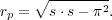
to be the mean distance to the pair. The separation between the two
galaxies across (rp) and along
( ) the line of sight are
defined as
) the line of sight are
defined as
 |
(13) |
 |
(14) |
One can then compute pair
counts over a two-dimensional grid of separations to estimate
(rp,
).
(s),
the one-dimensional redshift space correlation
function, is then equivalent to the azimuthal average of
(rp,
).
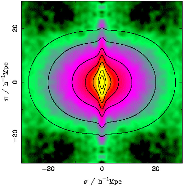 |
Figure 5. The two-dimensional redshift
space correlation function from 2dFGRS
(Peacock et
al. 2001).
Shown is
|
An example of a measurement of
(rp,
) is shown
in Fig. 5. Plotted is
as a function
of separation rp (defined in this figure to be
 ) across and
along the
line of sight. What is usually
shown is the upper right quadrant of this figure, which here has been
reflected about both axes to emphasize the distortions. Contours of
constant
follow the color-coding, where yellow corresponds to
large values
and green to low values. On small scales across
the line of sight (rp or
< ~ 2
h-1 Mpc) the contours are
clearly elongated in the
direction; this reflects the "Fingers
of God" from galaxies in virialized overdensities. On large scales
across the line of sight (rp or
> ~ 10
h-1 Mpc) the
contours are flattened along the line of sight, due to "the Kaiser
effect". This indicates that galaxies on these linear scales are
coherently streaming onto structures that are still collapsing.
) across and
along the
line of sight. What is usually
shown is the upper right quadrant of this figure, which here has been
reflected about both axes to emphasize the distortions. Contours of
constant
follow the color-coding, where yellow corresponds to
large values
and green to low values. On small scales across
the line of sight (rp or
< ~ 2
h-1 Mpc) the contours are
clearly elongated in the
direction; this reflects the "Fingers
of God" from galaxies in virialized overdensities. On large scales
across the line of sight (rp or
> ~ 10
h-1 Mpc) the
contours are flattened along the line of sight, due to "the Kaiser
effect". This indicates that galaxies on these linear scales are
coherently streaming onto structures that are still collapsing.
As this effect is due to the gravitational infall of galaxies onto
massive forming structures, the strength of the signature depends
on  matter.
Kaiser (1987)
derived that the large-scale anisotropy in
the (rp,
) plane depends on
matter.
Kaiser (1987)
derived that the large-scale anisotropy in
the (rp,
) plane depends on

 matter
/ b on linear scales,
where b is the bias or
the ratio of density fluctuations in the galaxy population relative to
that of dark matter (discussed further in the next section below).
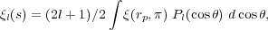
Anisotropies are quantified using the multipole moments of
(rp,
), defined as
matter
/ b on linear scales,
where b is the bias or
the ratio of density fluctuations in the galaxy population relative to
that of dark matter (discussed further in the next section below).
Anisotropies are quantified using the multipole moments of
(rp,
), defined as
 |
(15) |
where s is the distance as measured in redshift space,
Pl are Legendre polynomials, and
 is the angle between
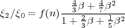
s and the line of sight. The ratio
2 /
0,
the quadrupole to monopole moments of the
two-point correlation function, is related to
in a simple
manner using linear theory
(Hamilton 1998):
is the angle between
s and the line of sight. The ratio
2 /
0,
the quadrupole to monopole moments of the
two-point correlation function, is related to
in a simple
manner using linear theory
(Hamilton 1998):
 |
(16) |
where f(n) = (3 + n) / n and n is the
index of the two-point correlation function in a power-law form:
 r-(3+n)
(Hamilton 1992).
r-(3+n)
(Hamilton 1992).
Peacock et al. (2001)
find using measurements of the
quadrupole-to-monopole ratio in the 2dFGRS data (see
Fig. 5) that
= 0.43
± 0.07. For a bias value of around unity (see
Section 5 below), this implies a low value of
matter ~
0.3. Similar measurements have been made with clustering measurements using
data from the SDSS. Very large galaxy samples are needed to detect
this coherent infall and obtain robust estimates of
. At
higher redshift,
Guzzo et al. (2008)
find =
0.70 ± 0.26 at z = 0.77
using data from the VVDS and argue that measurements of
as a
function of redshift can be used to trace the expansion history of the
Universe. We return to the discussion of redshift space distortions
on small scales below in Section 6.3.
What is often desired, however, is a measurement of the real space
clustering of galaxies. To recover
(r) one
can then project
(rp, ) along the rp axis. As redshift space
distortions affect only the line-of-sight component of
(rp,
), integrating
over the direction
leads to a statistic wp(rp), which
is independent of redshift space distortions. Following
Davis & Peebles
(1983),
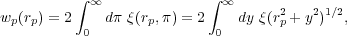 |
(17) |
where y is the real-space separation along the line of sight. If
(r) is
modeled as a power-law,
(r)
= (r / r0)- ,
then r0
and can
be readily extracted from the projected correlation
function, wp(rp), using an analytic
solution to Equation 17:
,
then r0
and can
be readily extracted from the projected correlation
function, wp(rp), using an analytic
solution to Equation 17:
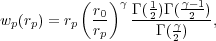 |
(18) |
where Γ is the usual gamma function. A power-law fit to
wp(rp)
will then recover r0 and
for the
real-space correlation function,
(r). In
practice, Equation 17 is not integrated to
infinite separations. Often values of
max are ~ 40-80
h-1 Mpc, which includes most correlated pairs. It is
worth noting that the values of r0 and
inferred are covariant. One must
therefore be careful when comparing clustering amplitudes of different
galaxy populations; simply comparing the r0 values may be
misleading if the correlation function slopes are different. It is
often preferred to compare the galaxy bias instead (see next section).
As a final note on measuring the two-point correlation function, as can
be seen from Fig. 3, flux-limited
galaxy samples contain a higher density
of galaxies at lower redshift. This is purely an observational artifact,
due to the apparent magnitude limit including intrinsically lower luminosity
galaxies nearby, while only tracing the higher luminosity galaxies further
away. As discussed below in Section 6, because the clustering amplitude of
galaxies depends on their properties, including luminosity, one would
ideally only measure
(r) in
volume-limited samples, where
galaxies of the same absolute magnitude are observed throughout the
entire volume of the sample, including at the highest
redshifts. Therefore often the full observed galaxy population is not
used in measurements of
(r),
rather volume-limited sub-samples are created where all galaxies are
brighter than a given absolute magnitude limit. This greatly facilitates
the theoretical interpretation of clustering measurements (see
Section 8) and the comparison
of results from different surveys.