


In this section, I will review some of the primary analysis techniques employed in IFS kinematic surveys at high-redshift. As can be seen from the discussion in the previous section, some of the key issues the surveys are tackling are:
Quantitative measurements are of course desirable and a variety of numerical techniques, many of which are new, have been devised to reduce IFS kinematic maps to a few basic parameters. All high-redshift observations are subject to limited signal:noise and spatial resolution, the best techniques allow for possible biases from such effects to be measured and corrected for — or be built in to the methodology.
Before launching in to the discussion of techniques, it is worth making some specific points about AO vs non-AO observations. While AO offers greater spatial resolution, a price is paid in the loss of light and signal:noise (for fixed integration times) through several principal effects:
Of course, AO observations reveal more about detailed structure resolving higher surface brightness features and for brighter more compact objects this can be critical for kinematic modelling and classification. Ideally one would use AO and natural seeing observations on the same objects and compare the results (e.g. Law et al. 2012a, Newman et al. 2013), discussed further in Section 5.2). Future work may combine both datasets, for example one can imagine a joint maximum-likelihood approach to disc fitting where the natural seeing data was used for faint, diffuse galaxy outskirts and complementary AO data used for the bright central regions.
As a first step (after data reduction to calibrated cubes), almost all analyses start out by making 2D maps of line intensity, velocity, and dispersion from 3D data cubes, this is a type of projection. The basic technique overwhelmingly used is to fit Gaussian line profiles in the spectral direction to data cube spaxels. The mean wavelength gives the velocity and the standard deviation the dispersion. The integral gives the line intensity. Typically, this can be done robustly when the integrated signal:noise (S/N) per resolution element being fitted is greater than a few, for example Förster Schreiber et al. (2009) used S/N > 5, Flores et al. (2006) used S/N > 3.
In order to estimate the dispersion map, it is necessary to remove the contribution from the instrument's spectral resolution. For resolved kinematics resolutions R ≳ 3000 are normally considered suitable (noting this is independent of redshift). Normally the instrumental resolution is subtracted 'in quadrature', meaning:
 |
(2) |
(e.g. Swinbank et al. 2012b) which is formally correct as the two broadenings are independent. However, in the case of low signal:noise and/or low dispersion this becomes problematic, if the best fit has σobs < σinstr due to noise then the quadratic subtraction can not be done, and when this happens it is ill-defined. A better approach that avoids this problem (Förster Schreiber et al. 2009, Davies et al. 201, Green et al. 2013) is to start with a model instrumental line profile, and broaden it by convolving it with Gaussians of different σgal (constrained to be > 0) until a good fit to the observed profile is achieved. This can also handle non-Gaussian instrumental profiles and gives more realistic errors.
Of course, making projections necessarily loses some of the information in the original cube, for example asymmetries and non-Gaussian wings on line profiles which can convey additional information on instrumental effects (such as beam-smearing) as well as astrophysical ones (such as infalls and outflows of material). At high-redshift, lack of signal:noise means these higher order terms can't currently be measured well anyway for individual spatial elements, however with future instruments and telescopes this will not remain true.
4.2. Measuring rotation curves
For galaxies identified as discs from kinematic maps, perhaps the most important kinematic measurement is to fit a model velocity field to extract rotation curve parameters. This allows construction of the Tully-Fisher relation at high-redshift for comparison with models of disc galaxy assembly.
In samples of nearby galaxies with long-slit optical observations, rotation curves with high-spatial resolution are constructed piecewise (i.e. binned velocity vs coordinate along the slit axis); the maximum velocity can be either read of directly (e.g. Mathewson et al. 1992) or a rotation curve model is fitted to it (i.e. a V(r) function) (e.g. Staveley-Smith et al. 1990, Courteau 1997, Catinella et al. 2005). There is a necessary assumption that the slit is along the principal kinematic axis. For 2D IFS observations (radio HI or Fabry-Perot emission line cubes in the early days) the 'tilted ring' approach has become standard (e.g. Rogstad et al. 1974, Schommer et al. 1993), where each ring measures the velocity at one radius and also represents a piecewise approach. At high-redshift, different approaches have been used primarily due to two factors (i) the lower signal:noise does not allow complex models with numerous parameters to be fit and (ii) the limited spatial resolution (often 5-10 kpc for a natural seeing PSF at z > 1) means 'beam smearing' effects are more severe and comparable to the scale of the underlying galaxy itself.
A standard approach to fitting 'rotating disc models' to 2D IFS data of high-redshift galaxies has emerged and been adopted by different groups and the essentials consist of:
This approach was originally developed for fitting long-slit data of high-z galaxies (see Section 2) and was an outgrowth of similar techniques being used in 2D galaxy photometry with the Hubble Space Telescopes (Schade et al. 1995).
The key advantage of this approach is the explicit inclusion of beam-smearing via the PSF convolution step, this leads to more unbiased best fit parameters. However, it is necessary to assume an underlying photometric model because the convolution with the PSF will mix velocities from different parts of the galaxy according to their relative luminosity.
The largest disc galaxies at high-redshift have effective radii of 5-8 kpc (Labbé et al. 2003, Buitrago et al. 2008), comparable to typical natural seeing PSFs, however the exponential profile is relatively slowly declining so that useful signal:noise is obtainable on scales of 2-3 arcsec, this is why the method works. AO data provides higher spatial resolution but at a considerable cost in signal:noise. Natural seeing data has proved surprisingly more successful than AO in revealing discs at high-redshift and it is thought this is due to its greater sensitivity to extended lower surface brightness emission at the edges of galaxies. The most successful AO projects have used very long exposures (> 5 h per source). That said, it can been seen that there are numerous galaxies at high-redshift that do not show rotation, and these may simply be instances whereas they are too small compared to natural seeing to resolve and too faint to be accessible to AO.
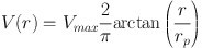
Variations on this core technique abound and is useful to review them. First, there is the choice of V(r) function. The two most commonly used analytic choices for high-redshift analyses are (i) the 'arctan' function:
 |
(3) |
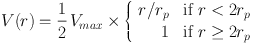
of Courteau (1997) which is an analytic form that expresses a profile initially rising smoothly with a 'kinematic scale radius' rp (Weiner et al. 2006a, Puech et al. 2008) and smoothly transitioning to a flat top; and (ii) the linear ramp function:
 |
(4) |
which has a sharp transition 16 (Wright et al. 2009, Epinat et al. 2012, Swinbank et al. 2012b, Miller et al. 2011). Both have exactly two free parameters though the ramp model better fits artificially redshifted simulations of high-redshift galaxies (Epinat et al. 2010) as it reaches its asymptote faster. Usage of the ramp function does make it clearer if the presence of any turnover (i.e Vmax) is well constrained by the data.
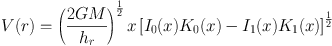
The other common approach to V(r) is to assume a mass model, usually a thin exponential disc, and integrate this up (Cresci et al. 2009, Gnerucci et al. 2011b). The solution for an ideal infinitely thin exponential disc is given by Freeman (1970b) (his Equation 12 and Figure 2) in terms of modified Bessel functions of the first (In) and second kind (Kn):
 |
(5) |
where M is the disc mass, hr is the disc scale length, and x = r / 2 hr. This has a maximum velocity peak (with a shallow decline at large radii) at 2.15 hr which is commonly called 'V2.2' and V2.2 / 2 occurs at 0.38 hr. More complex functions can arise from multiple components, for example at low-redshift the 'Universal Rotation Curve' formula of Persic et al. (1996) approximates an exponential disc + spherical halo and they arrive at a luminosity dependant shape. 17 The large velocity dispersions at high-redshift also motivates some authors to include this support in relating the mass model to the rotation curve (e.g. Cresci et al. 2009).
These variations can cause issues when trying to consistently compare Tully-Fisher relationships, for example some authors may choose the arctan function but then evaluate it at 2.2 scale lengths (e.g. Miller et al. 2011). Finally I note that it is often useful to fit a pure linear shear model (i.e. like a ramp functions but with no break) (Law et al. 2009, Wisnioski et al. 2011, Epinat et al. 2012). Because it has one less free parameter, it does not need a centre defined, and is not changed by beam-smearing it can be very advantageous for low signal:noise data and as a means of at least identifying candidate discs (see Section 4.5).
The choice of underlying photometric model is also important, because of the PSF convolution this affects how much velocities in different parts of the galaxy are mixed in the observed spaxels. An accurate PSF is also obviously vital and this can be problematic for AO data. Since the kinematics is being measured in an emission line such as Hα then one needs to know the underlying Hα intensity distribution to compute this correctly — however, this is not known as one only observes it smoothed by the PSF already so this is essentially a deconvolution problem. Most authors simply assume the profile is exponential (which may be taken from the IFS data or separate imaging) which is potentially problematic as we know high-redshift galaxies have clumpy star-formation distributions and possibly flat surface brightness profiles (Elmegreen et al. 2004b, Elmegreen et al. 2005, Wuyts et al. 2012). It may not make much of a difference if the galaxy is only marginally resolved as the PSF (which is much larger than the clump scale) dominates for natural seeing data (but see Genzel et al. 2008 who investigate and compare more complex M(r) mass models with the best resolved SINS galaxies). A different, arguably better, approach is to try and interpolate the intensity distribution from the data itself (Epinat et al. 2012, Miller et al. 2011). The photometric profile is also usually used to estimate the disc inclination and orientation for the deprojection to cylindrical coordinates, this is ideally done from HST images but is sometimes done from the projected data cube itself. Trying to determine the inclination from the kinematics is particularly problematic (though Wright et al. 2009 and Swinbank et al. 2012b do attempt this) as there is a strong near-degeneracy between velocity and inclination. One can only measure the combination V sin(i) except in the case of very high signal:noise data where the curvature of the 'spider diagram' becomes apparent (a well known effect, e.g. Begeman 1989 Section A2). I demonstrate this explicitly in Figure 9. The final key choice is the matter of which data is used for the fitting process. Obviously one must use the velocity map and associated errors, and most authors simply use that with a χ2 or maximum likelihood solver. One also normally has a velocity dispersion map and can also use this (Cresci et al. 2009, Weiner et al. 2006a), the dispersion maps contains information which constrains the beam-smearing (via the PSF convolution); however, one must make additional assumptions about the intrinsic dispersion (e.g. that it is constant). This case arises naturally if using a dispersion-supported component in a mass model.
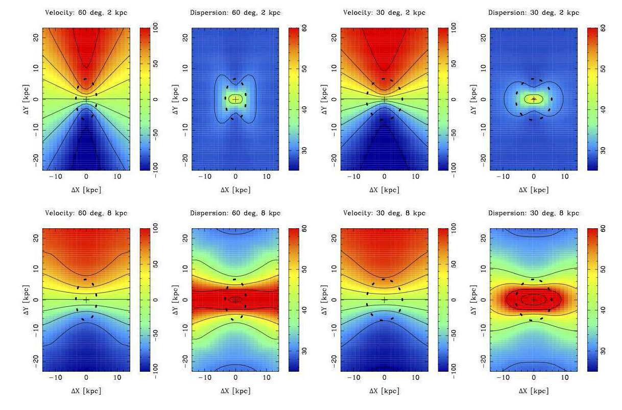 |
Figure 9. Model disc galaxy velocity and dispersion fields at inclinations of 30∘ and 60∘. The assumed galaxy model is an exponential disc in Hα emission with scale length h = 3 kpc (the heavy dashed ellipse shows the extent at 2.2h) and a rotation curve taken from Equation 3 with rd = 1 kpc. The top row is for a spatial resolution of 2 kpc (i.e the FWHM of a Moffat PSF) and the bottom row is for 8 kpc (a coarse resolution representing typical z > 1 natural seeing observations) and the intrinsic spectral resolving power is 7000. Models at different inclinations are defined to have constant Vmax sini = 110 km s-1 to illustrate this approximate degeneracy in velocity maps and the intrinsic dispersion is 20 km s-1. Contours run linearly from -100 to +100 km s-1 in velocity (25 km s-1 steps) and 30 to 70 km s-1 in dispersion (10 km s-1 steps). Note that the maps are projected from the underlying 3D disc model by fitting Gaussians to the spectral line profile as is standard for IFS observations, the high dispersion central peak is the result of beam-smearing, which is significantly worse at 8 kpc resolution, and the elongated high-dispersion bar arises from the Gaussian being a poor representation of the beam-smeared line shape. This can be accounted for in 3D disc fitting (i.e. summing χ2(RA,DEC,λ)) and this is in fact done by the code used to produce this figure. Credit: kindly provided by Peter McGregor (2013). |
Fitting disc models of course requires well-sampled high signal:noise data and of course the model needs to fit. With noisier data, fitting shears is a simpler approach, another simple parameter is to simply recover some estimate of Vmax from the data cube (Law et al. 2009, Förster Schreiber et al. 2009). If we expect discs to have a flat rotation curves in their outskirts then the outer regions will reproduce this maximum value with little sensitivity to exact aperture. Often the maximum pixel or some percentile is used. One also knows that for a random distribution of inclinations <V sini> = <V> <sini> and sini is uniformly distributed with an average of π/4 (Law et al. 2009). However, the use of a maximum may be subject to pixel outliers and the use of a limiting isophote may not reach the turnover (this is true for model fitting too but at least one then knows if one is reaching sufficiently far out). An unusual hybrid approach to fitting adopted by the IMAGES survey (Puech et al. 2008) motivated by their relatively coarse IFS sampling was to estimate Vmax from essentially the maximum of the data within the IFU, but use model fitting to the velocity map to calculate a correction from the data maximum to Vmax which they justified via a series of simulations of toy disc models.
All the papers in the literature have fit their disc models to 2D projections such as the velocity map; however, in principle it is possible for perform the same fitting in 3D to the line cube. This may provide additional constraints on aspects such as beam-smearing via the line profile shape (e.g. beam-smearing can induce asymmetries and effects in projection as is shown in Figure 9). This last approach has been tried in radio astronomy on HI data of local galaxies but is computationally expensive (Józsa et al. 2007). Fitting algorithms also require a good choice of minimisation algorithm to find the lowest χ2 solution given the large number of free parameters. Commonly steepest descent type algorithms are used; Cresci et al. (2009) used the interesting choice of a genetic algorithm where solutions are 'bred' and 'evolved'. (Wisnioski et al. 2011) used a Monte-Carlo Markov Chain approach which allows an efficient exploration of the full probability distribution (and marginalization over uninteresting parameters). In my view, this approach, which is common in for fitting cosmological parameters, is potentially quite interesting for future large surveys as in principle it could allow errors from individual galaxies to be combined properly to compute global quantities such as the circular velocity distribution function.
Given the variety of choices in disc fitting approaches by different authors, it is desirable to compare these using simulated galaxies and/or local galaxies (with well-measured kinematics) artificially degraded to simulate their appearance at high-redshift and explore systematics such as PSF uncertainty. This has not been done comprehensively, but a limited comparison was done by Epinat et al. (2010) using data from a local Fabry-Perot survey in Hα of UGC galaxies and simulating their appearance at z = 1.7 in 0.5 arcsec seeing; however, this was primarily focussed on evaluating beam-smearing effects. They did conclude that the galaxy centre and inclination are best fixed from broad-band high-resolution imaging and that using the simple ramp model statistically recovered reliable Vmax values more often than other techniques for large galaxies (size > 3× seeing). They also argue that the velocity dispersion map adds little constraining power to the disc fit.
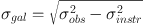
In the absence of 2D kinematic data and modelling, the 'virial estimator' for dynamical mass:
 |
(6) |
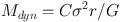
where σ is the integrated velocity dispersion and r is some measure of the size of the object has often been used (Erb et al. 2006b, Law et al. 2009, Förster Schreiber et al. 2009, Lemoine-Busserolle & Lamareille 2010). In this case, σ represents unresolved velocity contributions from both pressure and rotational support and C is a unknown geometric factor of O(1) (C = 5 for a uniform rotating sphere, Erb et al. 2006b). This is cruder than 2D kinematics in that kinematic structure and galaxy inclination are ignored, in a sense the goal of 2D kinematics is to reliably measure C. However it can be applied to larger samples.
A related novel method is the use of the technique of 'spectroastrometry' to measure the dynamical masses of unresolved objects. This technique was originally developed to measure the separations of close stellar pairs (Bailey 1998) and allows relative astrometry to be measured at accuracies very much larger than the PSF limit. In the original application, it relies on measuring the 'position spectrum', i.e. the centroid of the light along the long-slit as a function of wavelength. As one crosses a spectral line, with different strengths and shapes in the two unresolved stars, one measures a tiny position offset. Because this is a differential technique as very close wavelengths systematic effects (e.g. from the optics, the detector and the PSF) cancel out and the measurement is essentially limited by the Poisson signal:noise ratio. Accuracies of milli-arcsec can be achieved in natural seeing. Gnerucci et al. (2010) developed an application of spectroastrometry for measuring the masses of black holes and extended this (Gnerucci et al. 2011a) to galaxy discs in IFS measurements. The technique here now involves the measurement of the position centroid (now in 2D) of the blue vs red half of an emission line as defined by the integrated spectrum and mean wavelength. In the presence of rotation, there is a small position shift. Unlike stars galaxies are complex sources and there can be systematic effects, for example if the receding part of the disc has a different clumpy Hα distribution than the approaching part. The classical Virial mass estimator (Mdyn ~ r σ2 / G) requires a size measurement r which is difficult for unresolved compact objects and is often taken from associated HST imaging for high-redshift galaxies; this gets replaced by the spectroastrometric offset rspec. Gnerucci et al. find the spectroastrometric estimator gives much better agreement (~ 0.15 dex in mass) than the virial estimator for high-redshift galaxies with good dynamical masses from 2D modelling. They also argue from simulations that it ought to work well for unresolved, compact galaxies. It is certainly a promising avenue for further work and could help, in my view, resolve the nature of dispersion-dominated compact galaxies. Spectroastrometric offsets do require modelling to interpret, however the presence of a position offset is a robust test for the presence of unresolved shear irrespective of a model.
4.4. Velocity dispersion Measures
A key discovery is that is has been consistently found that high-redshift galaxies have higher intrinsic (i.e. resolved) velocity dispersions than local galaxy discs. 18 Thus, it is necessary to reliably measure this quantify, and in particular derive some sort of 'average' from the kinematic data. In fact, one approach has been to define a simple average:
 |
(7) |
over the pixels, as used in Gnerucci et al. (2011b), Epinat et al. (2012). One can also define a flux or luminosity weighted average:
 |
(8) |
(Law et al. 2009, Green et al. 2010) which is less sensitive to low S/N pixels and exact definition of outer isophotes.
The observed dispersion will include a component of instrumental broadening which must be removed (see Section 4.1) but will also include a component from unresolved velocity shear (such as might be caused by systematic rotation). The PSF of the observation will cause velocities from spatially nearby regions to be mixed together and if these are different then this will show up as an increased velocity dispersion called 'beam-smearing'. This will get worse for spatial regions with the steepest velocity gradients and for larger PSFs. Brighter spatial regions will also dominate over fainter ones so the effect also depends on the intrinsic flux distribution. One method to correct for this beam smearing is to try and compute a 'σ from beam-smearing' map from the intensity/velocity maps (interpolated to higher resolution) and then subtracting this in quadrature from the observed map (Gnerucci et al. 2011b, Epinat et al. 2012, Green et al. 2010). Use of σm and σa has the advantage that they are non-parametric estimators and have meaning even when the dispersion is not constant (i.e. they are averages).
Another approach to calculating the intrinsic dispersion is to incorporate it in to the disc modelling and fitting approaches discussed in Section 4.2. For example, in their dynamical modelling, Cresci et al. (2009) incorporated a component of isotropic dispersion (they denote this the 'σ02' parameter), which they then fit to their velocity and velocity dispersion maps jointly. In this way, the PSF and the beam-smearing are automatically handled as it is built in to the model. Their model maps are effectively constant and ≃ σ02 except in the centre where there is a dispersion peak due to the maximum velocity gradient in the exponential disc model (e.g. see Figure 4 examples).
Davies et al. (2011) compared these different approaches to calculating dispersion using a grid of simulated disc galaxies observed at different spatial resolutions (and inclination etc.) similar to high redshift surveys. In particular, they concluded that the method of empirically correcting from the intensity/velocity map is flawed as that map has already been smoothed by the PSF,which leads to less apparent shear than is really present, and that the σm and σa type estimators are highly biassed even when corrected. They also concluded that the disc fitting approach was the least biased method for estimating σ. However, I note that the underlying toy disc model used for the simulated data closely agrees with the model fitted to the data by construction, so this is not in itself surprising. A parametric approach such as fitting a disc with a constant dispersion may also be biased if the model assumptions are wrong — for example, if the dispersion is not in fact constant or the rotation curve shape is incorrect. It is clear though that use of σm in particular should be with extreme caution as it is one of the most sensitive of the dispersion estimators to beam smearing in high-shear galaxies. The parametric approaches tend to underestimate the dispersion at low signal:noise and the non-parametric ones to over-estimate it. The dispersion measures of Green et al. (2010), Gnerucci et al. (2011b) and Epinat et al. (2012) may be biased by the effect Davies et al. discusses, the degree to which will depend on how well the parameters of the galaxies in question reproduce those chosen in the simulations of Davies et al. and this is yet to be quantified.
4.5. The merger/disc classification
One early goal of high-redshift IFS surveys was to try and kinematically distinguish modes of star-formation in high-redshift galaxies. It was already known that star-formation rate was typically factors of ten or more higher at 1 < z < 4 than locally (Madau et al. 1996, Lilly et al. 1996), and that massive galaxies (~ 1011 M⊙) in particular were much more actively forming stars (Bell et al. 2005, Juneau et al. 2005). Models of hierarchical galaxy assembly a decade ago were typically predicting that mergers (as opposed to in-situ star-formation) were the dominant source of mass accretion and growth in massive high-redshift galaxies (Somerville et al. 2001, Cole et al. 2000). Is it possible that the increase in cosmic star-formation rate with lookback time is driven by an increased rate of merger-induced starbursts?
In photometric surveys on-going mergers have been identified by irregular morphology (Conselice et al. 2003, Conselice et al. 2008, Bluck et al. 2012), however this is not always definite because as we will see in Section 5.1 it is now established that many disc-like objects at high-redshift appear photometrically irregular as their star-formation is dominated by a few large clumps embedded in the discs. Thus, it is desirable to additionally consider the kinematics. Another popular technique has been to count 'close pairs' in photometric surveys and/or redshift surveys (i.e either 'close' in 2D or 3D) and then calibrate how many of them are likely to merge on a dynamical time scale via simulations (Lotz et al. 2008, Kitzbichler & White 2008). This technique may fail for a late stage merger when the two components are not well separated any more.
A number of techniques have been used to try and differentiate between galaxy-galaxy mergers and discs in kinematic maps. As can be seen from Section 3, some high-redshifts surveys have found up to a third of their targets to have merger-like kinematics so this is an important issue.
The first and most widely used technique is simply visual classification using either the velocity and/or dispersion maps. One expects a disc to have a smoothly varying clear dipolar velocity field along an axis, and to be symmetric about that axis. At high signal:noise, one would see a 'spider diagram' type pattern. The dispersion field would also be centrally peaked if the rotation curve was centrally steep and beam-smearing was significant. One might expect a merging second galaxy component to distort the motions of the disc, one would also expect to see a discontinuous step in the velocity field when one transitions to where the second galaxy dominates the light. A good example of a z = 3.2 merger with such a step is shown in Nesvadba et al. (2008) - their Figure 3. 19 Such visual classifications have been used in Yang et al. (2008), Förster Schreiber et al. (2009) and Law et al. (2009). Of course, such visual classifications are subjective and also susceptible to signal:noise/isophote levels. In imaging surveys, the equivalent 'visual morphologies' have often been exhaustively tested by comparing different astronomer's classifications against each other and against simulations as a function of signal:noise, this has not yet been done for kinematic classifications.
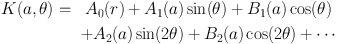
Turning to algorithmic methods to classify galaxy kinematics, the most popular technique has been that of 'kinemetry' (the name is an analogy of 'photometry') which tries to quantify asymmetries in velocity and dispersion maps. Originally developed by Krajnović et al. (2006) this was used to fit high signal:noise local elliptical galaxy IFS observations, but has been adapted to high-redshift z ~ 2 SINS discs by Shapiro et al. (2008). By analogy to surface photometry kinemetry proceeds to measure the 2D velocity and velocity dispersion maps using azmimuthal kinematic profiles in an outward series of best fitting elliptical rings. The kinematic profile as a function of angle θ is then expanded harmonically. For example:
 |
(9) |
where a would be the semi-major axis of the ellipse (which defines θ = 0). This is of course equivalent to a Fourier transformation, the terms are all orthogonal. When applied to an ideal disc galaxy we expect (i) the velocity field should only have a single non-zero B1 terms since due to its dipolar nature it goes to zero at θ = ± π / 2, with B1(a) representing the rotation curve (ii) similarly the symmetric dispersion map should only have a non-zero A0(a) term representing the dispersion profile. When higher terms are non-zero, these can represent various kinds of disc asymmetries (bars,warps, etc.) or just arise from noise. The primary difference between the high signal:noise local application and the low signal:noise high-redshift application of Shapiro et al. is that in the latter a global value of the position angle and inclination (ellipticity) is solved for instead of allowing it to vary in each ring. These are found by searching over a grid of values to find those which essentially minimise the higher-order terms.
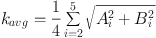
Shapiro et al. expanded their kinemetry to fifth order and in particular defined an average power in higher-order coefficients (which should be zero for a perfect disc) as
 |
(10) |
then they defined velocity and dispersion asymmetry parameters as
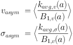 |
(11) (12) |
(where the second subscripts denote the relevant maps) that are normalised to the rotation curve (representing mass) and averaged across radii. The use of these particular parameters was justified by a series of simulations of template galaxies artificially redshifted to z ~ 2, these templates (13 total) included toy models of discs, numerical simulations of cosmological discs and actual observations (15 total) of local discs and ULIRG mergers. Figure 10 shows the location of these in the vasym, σasym diagram and Shapiro et al.'s proposed empirical division, represented by
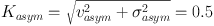 |
(13) |
 |
Figure 10. Kinemetry diagram classifying SINS galaxies. Axes are the velocity and dispersion asymmetry (as defined in the main text) with the line showing the proposed disc/merger boundary Kasym = 0.5. The points are the SINS objects classified by Shapiro with the outset velocity diagrams showing two sample objects classified as a disc (bottom object) and a merger (top object). Note how the disc shows a dipolar velocity field whereas the merger is more complex. The red/blue colour scale shows the probability distribution of simulated merger/disc objects at z ~ 2 (see Shapiro et al. for details). Credit: from Figure 7 of Shapiro et al. (2008), reproduced by permission of the AAS. |
Using this approach, Shapiro et al. successfully classified 11 of the highest signal:noise galaxies in the SINS samples (see Figure 10), and concluded that ≃ eight were discs and ≃ three were mergers (both ≃ ± 1), agreeing with visual classification. This kinemetry technique was also applied by Swinbank et al. (2012b) to their high-z sample and they also did an independent set of simulations to verify the Kasym < 0.5 criteria and found a 55% disc fraction. Gonçalves et al. (2010) applied this to their sample of z ~ 0.2 compact dispersion-dominated 'LBAs' (see Section 3.9), both as observed and when artificially redshifted to z = 2.2 (specifically simulating SINFONI in natural 0.5 arcsec seeing). They found a 'merger' fraction (Kasym > 0.5) of ~ 70%, predominately for galaxies with stellar masses < 1010 M⊙, but this dropped to ~ 40% for their high-redshift simulations, i.e. a large number of mergers were misclassified as discs, due mainly to the loss of visibility of outer isophotes and PSF smoothing. Of course these issues also affect visual classifications.
Alaghband-Zadeh et al. (2012) applied kinemetry to a sample of nine sub-mm galaxies at 2 < z < 2.7 observed with IFS. They found that essentially all of these were mergers with high asymmetries in both velocity and dispersion maps. Bellocchi et al. (2012) found that local LIRGS (two mergers and two discs) were reliably classified by kinemetry and simulated their appearance at high-redshift. They advocated a modified version of kinemetry where the ellipses were weighted by their circumference which gives more weight to the outer regions of the galaxies. An analysis of a larger number of 38 galaxies in this latter sample is forthcoming.
Some caveats are warranted, in my view particularly in the application of galaxy simulations to calibrate kinemetry. In the Shapiro et al. figure (Figure 10) and the other papers which use this classification diagram all the simulations are lumped together; however, it would be desirable to obtain a deeper understanding of the range of applicability by separating these out. For example, considering real galaxies and model galaxies separately, understanding the effects from the different kinds of simulation, how parameters degrade with signal:noise, the effects of choice of radial binning, inclination and resolution and so on. A paper exploring these in detail would be of great value to the literature.
A different approach to quantitative classification was used in the MASSIV survey (Epinat et al. 2012). They considered two classification parameters they derive from their disc fits. (i) the mean amplitude of the velocity residuals from the disc fits (normalised by the maximum velocity shear) and, (ii) the alignment between kinematic axes and photometric axes (determined from broad-band imaging). They identify an isolated cloud of points near the original with aligned axes (agreement < 20∘) and velocity residuals < 20% which they label 'rotators' and constituting half their sample. They argue the results are consistent with kinemetry, however no extensive set of simulations were done to establish the reliability. Dispersion information was not considered, they argued that the velocity and dispersion asymmetries are well correlated anyway (this is indeed evident in Figure 10) and of course Shapiro et al. did in fact combine these in to a single parameter.
Finally, I note that all these approaches are more or less parametric model-fit approaches 20 based on 2D projections, disc fitting plays a key role in that rejecting it is a basis for potential merger classifications. Kinemetry has similarities to non-parametric measures used in quantitative image morphology, especially in its use of an asymmetry measure which is similar to that used in morphology (Abraham et al. 1996b, Conselice 2003). However, model-fitting is still performed in order to determine a best fit inclination and PA before calculating the kinemetry coefficients. Soler & Abraham (2008, private communication) investigated the use of the Radon Transform to compute a statistic to distinguish model discs from mergers with some success. However, again this relies on statistics measured from 2D projections of the intrinsically 3D data. In principal, one can imagine deriving statistics from the 3D intensity emission line data cubes — a disc model makes a characteristic pattern of shapes in 3D position-velocity when viewed from different angles. However, to my knowledge no such approach has yet been undertaken in the literature; this is quite a contrast to 2D morphology where we have seen the use of a variety of statistics such as concentration, asymmetry, clumpiness, (Conselice 2003) 'M20' and Gini (Abraham et al. 2003, Lotz et al. 2004) has contributed to quantitative study of morphological evolution.
Regardless of the techniques used, it is clear that a substantial amount of further work is required to calibrate the quantitative application of these techniques at high-redshift. Also, it is desirable to move away from the simple 'merger vs disc' dichotomy which some authors have reasonably argued is an oversimplification (Wisnioski et al. 2011, Law et al. 2009) of continuous mass assembly by competing processes. It would be desirable to be able to apply quantitative techniques to estimate merger mass ratios and merger evolutionary stages (e.g. first approach, fly-by, coalescence as Puech et al. 2012 attempts visually) from IFS data, each of which have their own timescales, in order to test galaxy formation models.
4.6. Properties of substructures
As we will see in Section 5.1, the 'clumpy turbulent disc' model is emerging as a key paradigm to understanding the physical structures of at least some high-redshift galaxies as revealed by high-resolution imaging and IFS data (Elmegreen et al. 2004a, Elmegreen & Elmegreen 2005, Genzel et al. 2006, Elmegreen et al. 2009a, Bournaud et al. 2009, Genzel et al. 2011, Guo et al. 2012). In this scenario, large 'clumps' which are peaks of local emission are distinct physical structures in a galaxy disc and tests of the clump model involve measure of their resolved spatial and kinematic properties. Additionally, we have seen that some high-redshift objects are thought to be advanced stage mergers, in this case the sub-components may be distinct galaxies. I will briefly review some of the techniques used to define the physical properties of such substructures, the physical models will be discussed further in Section 5. It will be seen that the techniques used so far have been very basic and unlike the total galaxy measurements, absolutely require AO (or HST observations in the case of pure morphological work) as the 1-2 kpc scales need to be resolved. The extra resolution further provided by gravitational lensing (100-200 pc) has been especially critical in developing this area. I do not strictly consider IFS data in this section, but also imaging data as the techniques are in common.
A necessary starring point is identification of clumps. Often this is done by simple peak-finding codes, visual inspection or validation (Swinbank et al. 2009, Genzel et al. 2011, Wisnioski et al. 2012, Guo et al. 2012) as the number of individual clumps per galaxy is typically ~ 2-5. Of course the problem of identifying compact blobs against a background is a long studied one in astronomy and there has been considerable borrowing of well-established algorithms. In local galaxies, flux isophotes in Hα are often used to identify the numerous HII regions in nearby galaxies (Kennicutt et al. 1989); this has also been applied at high-redshift (Jones et al. 2010, Wuyts et al. 2012). More sophisticated techniques allow for a variable background, e.g. Förster Schreiber et al. (2011) applied the star-finding software daofind (Stetson 1987) to HST infrared images, looking for local maxima above a background threshold and validated visually, to find 28 clumps in six z ~ 2 galaxies. If clumps are resolved then star-finders may not be appropriate, especially if they assume point sources with a particular PSF, because of this (Livermore et al. 2012) adopted the clumpfind program (Williams et al. 1994) (albeit in a 2D mode for their HST images) originally developed for the analysis of molecular line data in the Milky Way. This proceeds by thresholding at a series of progressively fainter isophotes to try and deblend overlapping clumps. Resolution effects are an issue — if we looked at a grand design spiral with resolution of only 1 kpc, would we see the numerous HII regions in the spiral arms merge together to make only a few larger single objects? The answer so far appears to be subtle: Swinbank et al. (2009) did simulations of this effect using local galaxies and found such 'region merging' did indeed result in few regions of greater size and luminosity. They argued the vector of this change was nearly parallel to the existing size-luminosity relation and did not result in an offset relation as they found at high-redshift. A similar effect was found in Livermore et al. (2012), noting that the magnitude of the effect (vector A in their Figure 6) is approximately a factor of two in size and luminosity. Both of these particular studies were being compared to lensed high-redshift sources where the resolution was ~ 300-600 pc and the clump radii up to a kpc.
The method of measuring clump sizes is also an issue. The traditional approach in local galaxy studies is after finding HII regions through an isophotal selection to simply define the radius as √Area /π, i.e. the radius of a circularised region. The other approach is to fit profiles to the regions and then use the half-width at half maximum (HWHM) as the size, this is known as the 'core method' (Kennicutt 1979). Isophotal sizes are problematic in that they depend on the exact isophote chosen, and often it is not a defined physical surface brightness in Hα but simply a signal:noise level (e.g. Jones et al. 2010). In this case, just taking deeper data will result in larger sizes. Compared to a faint region a region with a higher luminosity but the same core radius will have a larger isophotal radius, this is particularly problematic when comparing different redshifts as there will be a degeneracy between luminosity and size evolution in region properties. Wisnioski et al. (2012) and Livermore et al. (2012) both considered the effect of the choice of core vs isophotal radii. Wisnioski et al. (2012) found the isophotal radiii in their local galaxy comparison samples were up to three times larger than core radii (determined by fitting 2D gaussians) and attributed this to the inclusion of diffuse emission in isophotes; in contrast, the respective luminosities were much more in agreement as they are dominated by the brighter inner parts. They argued that core radii were a more robust choice for high-redshift comparisons. Livermore et al. (2012) found good agreement between clump sizes at high-redshift from clumpfind isophotes and core sizes (for sizes > 100 pc).
Both types of radii are subject to resolution effects which clearly need to be simulated and this has been done by several groups (Elmegreen et al. 2009a, Swinbank et al. 2009, Livermore et al. 2012). Even for nearby galaxies this may be critical, for example Pleuss et al. (2000) studied resolution effects in M101 comparing HST data of this nearby galaxy to simulated natural seeing at a distances several times greater. They found the effect of changing the resolution from 4 pc up to 80 pc (still much better than typical high-redshift data) was to merge regions due to their natural self-clustering and boost their isophotal sizes by factors of 2-4 . They even hypothesised that the 'break' in the HII region Hα luminosity function at ~ 1039 ergs s-1 (Rozas et al. 1996) could be entirely due to resolution effects in typical local data. The largest and most luminous HII regions with sizes of up to 300 pc were the least effected by the degradation, as might be expected, this conclusion echoes the earlier work of Kennicutt et al. (1989). More systematic studies of the effect of resolution on size measurements at high-redshift is clearly needed; existing work only treats this topic briefly on the way to the high-redshift results of interest. There is clearly a problem: for example Figure 6 of Livermore et al. (2012) suggests there is a factor of 10 vertical offset between the nearby and z ~ 1 luminosity-size diagram of clumps (see also Swinbank et al. 2009, Jones et al. 2010). However, Wisnioski et al. (2012) (their Figure 6) argues that there is a single relation. This large difference seems to arise from the use of isophotal vs core sizes. Another potential issue is that a significant number of the size measurements in the literature exploit the extra magnification due gravitational lensing (Swinbank et al. 2009, Jones et al. 2010). This of course allows smaller physical scales to be resolved but it should be noted that the magnification is very anamorphic and the extra resolution is only attained in one spatial dimension.
The topic of clump velocity and velocity dispersion has cropped up in a few papers. Generally, dispersion is normally measured from the integrated spectrum in an aperture at the position of the clump and can be used to estimate scaling relations and derive Jeans masses (Swinbank et al. 2009, Genzel et al. 2011, Wisnioski et al. 2012). Clumps share the velocity field of the underlying galaxy disc; this in fact is a key test of the clump disc model. (If they were external merging galaxies one would expect a kinematic discrepancy and this is seen in these cases, e.g. Menéndez-Delmestre et al. 2013). They also seem to share the dispersion of the disc; at least distinct features (such as a peak or trough) are not apparent in dispersion maps at clump locations (for example see Figure 3 of Wisnioski et al. 2011, Figures 3-6 of Genzel et al. 2011 or Figure 4). One novel technique to investigate clump formation physics is to calculate spatial maps of the Toomre Q parameter under the expectation that clump locations might correspond to Q(RA,DEC) < 1). This requires a disc model velocity field and an inclination; I discuss the physical basis for this and potential problems of Q-maps further in Section 5.1. Clumps may also rotate internally and have significant dynamical support from this rotation and this is suggested by some simulations (Bournaud et al. 2007, Ceverino et al. 2012). This has been looked for by searching visually for apparent shears in residual velocity maps (after subtracting the best fitting disc model) with perhaps a tentative detection of small signals in some cases (Genzel et al. 2011); however they are small at the ~ 15 km s-1 kpc-1 level. One can also consider the application of resolved rotation curves to derive resolved mass profiles of galaxies at high-redshift. Kinematics of course can be sensitive to unseen components, for example evolved central bulges in disc galaxies may have no Hα emission but reveal themselves through their effect on rotation curves. There has been little of this in the high-redshift literature, probably because to do this properly requires AO observations and the number of AO samples is small and they only contain handfuls of galaxies. Genzel et al. (2008) present an application of this to the SINS survey (five galaxies which were the best observed, two with AO) where they extract a 'mass concentration parameter' defined as the ratio of total dynamical mass within the central 0.4 arcsec (3 kpc at z = 2) to the total (limited at 1.2 arcsec); the technique to derive this was to add Mdyn(0.4″) / Mdyn(1.2″) as an extra free parameter to the mass modelling of the 1D rotation curves along the major axis, holding the previously determined 2D disc fit parameters fixed. They do find an interesting correlation with emission line ratios in the sense that (their interpretation) more concentrated galaxies are more metal rich. One of their galaxies (BzK6004) shows high concentration and a beautiful detection of a central red bulge in the K-band continuum, surrounded by a clumpy Hα emitting disc. However, it is not clear in my view if 'mass concentration' in the sense defined on average means presence of a bulge or simply a more concentrated disc; and this would be a fruitful area to examine further with larger AO samples particularly looking at this type of modelling in more detail, with greater numbers and correlating with bulge presence (e.g. as revealed by HST near-infrared observations).
Finally, using IFS data one can measure other spectral, non-kinematic properties of galaxy sub-structures. Line luminosities and ratios can be measured by standard aperture photometry techniques. These can be used to derive physical properties such as star-formation rate and gas-phase metallicity in much the same way as for integrated spectra. These physical conversions can be complex and are beyond the scope of this review's discussion, for a thorough discussion of star-formation indicators see Hopkins et al. (2003) and for gas phase metallicity measurements, see Kewley & Ellison (2008).
16 In the way I have expressed both of these at rp the velocity is half of the maximum value. Back.
17 This dependence gives rise to circularity issues in Tully-Fisher applications (Courteau 1997). Back.
18 I re-emphasise that in this section I am not talking about dispersions of integrated spectra. Back.
19 One may also expect the spectral line ratios to change abruptly if, for example, the galaxies had different metallicities. Back.
20 Noting the key difference between parametric and non-parametric approaches is the assumption of an underlying parameterised model whose residuals are minimised with respect to the data. Back.